How to use Data Tables in Excel

Excel’s built-in Data Tables should be used when you want to show how changes in a particular input affect a key output, ie, you want to flex one variable (known as a “one-variable” or “one-dimensional” Data Table) or two variables (known as a “two-variable” or “two-dimensional” Data Table).

Being able to change one or two inputs at a time helps utilise Excel’s what-if? capabilities. Given the variables that may be changed directly using this feature (although data may be linked from elsewhere if required, so you have a “set” representing “scenario 1”, another representing “scenario 2”, etc.), Data Tables are highly useful when trying to understand the effects of certain key drivers of a model on a particular output. This is commonly known as sensitivity analysis (for changing one variable) or scenario analysis for changing multiple inputs concurrently in the modelling fraternity.

With this borne in mind, let’s take a look at each in turn. This Excel file provides examples to be viewed in conjunction with this article.

One-dimensional (1-D) Data Tables

This is best illustrated using an example — see the following screenshot:

It’s not vital you understand what this spreadsheet is doing. It is essentially using inputs in cells G10 and G15:L15 to generate an output in cell G29, as it calculates what cash received in row 15 would be worth now (the net present value, or NPV) if interest was 8% per period.

I appreciate this example could be constructed using the NPV function; however, I have displayed the calculation in clear steps, instead, to clearly highlight the benefits of using a Data Table.

Therefore, with a simple NPV calculated for a total of six periods (0 to 5 inclusive), the output for a discount rate of 8.0% (cell G10) is +$9,482 (cell G29).

But what if I wanted to know how the NPV would change if I varied the input discount rate?

It is very easy to construct a table (a Data Table) similar to the one displayed in cells E34:F46 above. First, the required discount rates are simply typed into cells E35:E46. The formula

=G29

then replaces the header in cell F34 (I note this no longer says “NPV”, but keep reading), then select cells E34:F46 and go to Data Table in the What-If Analysis drop-down menu in the Forecast grouping of the Data tab on the Ribbon (ALT+A+W+T) — see the screenshot below:

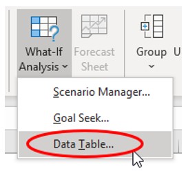
This calls the Data Table dialog box — see the screenshot below:

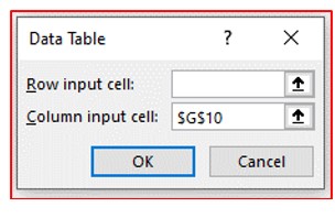
At this point, confusion often sets in as users are often unsure whether they should be entering details in the Row input cell: and/or Column input cell: input boxes. The rules are very simple:

• Referenced directly, the inputs and outputs must be on the same sheet as the Data Table (although there are ways and means around this).
• Use only one input box if you want to flex one input; use both if you wish to flex two.
• If inputs are in a column in the Data Table, use the Column input cell: input box.
• If inputs are in a row in the Data Table, use the Row input cell: input box.

Here, my inputs are in a column, and I want to use them to substitute for the value in cell G10 so I select cell G10 for the Column input cell: input box.

This provides the outputs varied by the given rates, but I need to fix cell F34.

For a 1-D Data Table to work using a columnar table similar to the one illustrated, the top row of the second and any subsequent columns have to contain the reference to the output cell(s). Many modellers will do this, putting the headings in the row above instead, and then they may or may not hide this row in order to compensate.

There is a crafty alternative (employed above). To begin, use CTRL+1, ALT+H+O+E, or select Format Cells from the Format drop-down menu in the Cells grouping of the Home tab of the Ribbon to reach the Format Cells dialog box. Then, if we go to the Number tab, we can keep the formula(s) but change the outward appearance of the cell. It is with this borne in mind that cell F34 is formatted as follows:

Here, I have typed in “NPV”;“NPV”. Essentially, what I have done here is replaced all non-negative numbers with the text “NPV” and negative numbers with the text “NPV”. You might wonder why I have I typed this in twice? If the number is negative and the second “NPV” has not been defined, the negative number would be replaced by “-NPV” instead — which is not what we want.

Having made this formatting modification, clicking OK results in the following summary:

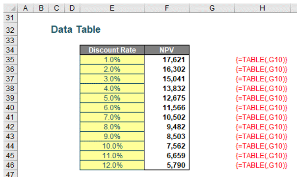
That’s it — you have your “What-if?” analysis. It should be noted that at this point, you may not enter any rows or columns into the Data Table (or delete any either). This is because the formula

{=TABLE(,G10)}

has been entered into cells F35:F46. The braces { and } may not need to be typed in. These are special characters created by Excel when you type the formula,

=TABLE(,G10)

and press CTRL+SHIFT+ENTER rather than ENTER. This is known as an array formula (albeit what is now known as a legacy array formula), and these cannot be edited, merely deleted in their entirety.

If the table had been across a row instead, ensure that the input values are in the top row and that the “headings” are in the first column (ie, transpose the example table, above). Then, you would populate the Row input cell: box instead.

1-D Data Tables do not need to be simply two columns or two rows. It is entirely possible to display the effects on more than one output at the same time — provided you wish to use the same inputs throughout the sensitivity analysis as follows:

Sometimes, you may find all of the numbers in your Data Table are identical. If this happens, you need to check your calculation settings. To do this, go to Excel Options (File -> Options or ALT+F+T) and then select Formulas. In the Calculation options section, please ensure the Workbook Calculation is set to Automatic — see the screenshot below:

In later versions of Excel, “Automatic except for data tables” has been replaced by “Partial” to cater for other features, such as Python in Excel.

Any other setting will not calculate Data Tables correctly. The reason for this is that Data Tables can consume a significant amount of memory and slow down workbook calculations — hence the options to disable them.

2-D Data Tables

2-D Data Tables are similar in idea: They simply allow for two inputs to be varied at the same time. Let’s extend the 1-D example as follows below:

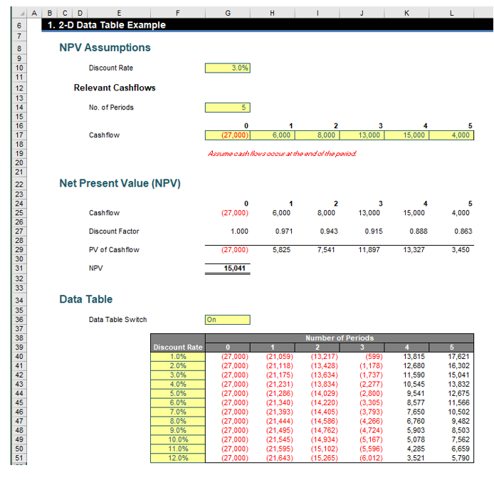
This example is similar but only calculates the NPV for a certain number of periods — specified in cell G14. Our 2-D Data Table (which is cells F39:L51, not F38:L51) can answer the question, “What is the NPV of our project over x periods with a discount rate of y%?”

If anything, a 2-D Data Table is simpler than its 1-D counterpart since there is little confusion over row and column input cells. Again, the output needs to be in the table, and this time it must be in the top left-hand corner of the array. In our example, it is disguised as “Discount Rate”, using similar number formatting to that described earlier. The formula in my example above employs:

=IF($G$36=”On”,$G$31,)

This allows for me to create a switch in cell G36, which allows me to toggle the Data Table off and on. This is an explicit way to prevent Data Tables from calculating rather than using the implicit approach detailed earlier in File -> Options.

The inputs required now form the remainder of the top row and the first column of the Data Table. With cells F39:L51 highlighted, the Data Table dialog box is opened as before — see the screenshot below:

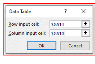
Since the top row contains the inputs for the number of periods, the Row input cell: should reference $G$14, whilst the discount rate inputs (Column input cell:) should link to $G$10 once more.

Once OK is clicked, the Data Table will populate as required — it’s simple.

Data Table inputs should be hard-coded

Don’t use formulas for inputs in either the first row or column of a Data Table. Let me explain why, by considering the following example:

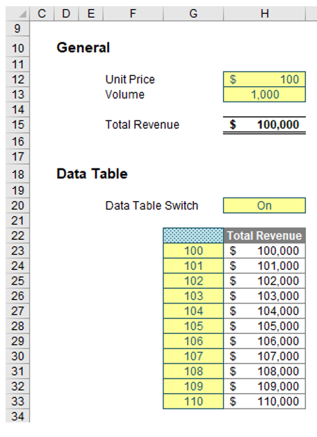
To be fair, this spreadsheet is arguably too simple to create a Data Table output, but I am using it to highlight the dangers of using formulas for inputs. In this example, all cells in yellow are inputs. The calculation in cell H15 is straightforward: =H12*H13. But that’s not the point here.

Cell H20 contains “On”, which is used for the formula in cell H22:

=IF(H20=”On”,H15,)

That is, the formula refers to the Total Revenue in cell H15 if the value in cell H20 is “On”, as before. The reason cell H22 appears to be a heading that says “Total Revenue” is we have used the number formatting (CTRL+1) trick again — see the screenshot below:

The Number formatting is Custom and has the key:

“Total Revenue”;”Total Revenue”

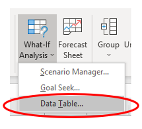
After the required input values (100 to 110 inclusive, as displayed) have been hard-coded into cells G23:G33, the range G22:H33 has been selected, and then a Data Table has been created by selecting Data Table… from the What-If Analysis drop-down menu in the Forecast group of the Data tab of the Ribbon — see below:

Since the inputs go down a column and the input cell is cell H12, the resulting Data Table dialog box has been populated thus:

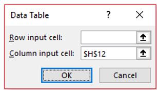
Assuming workbook calculations are set to Automatic (ALT+T+O), that’s all you have to do — it’s simple.

So, what’s the problem when inputs are formulaic? Consider this revised example below:

Here, the columnar inputs (cells G53:G63) have been replaced by a formula:

=IF(G52=””,$H$42,G52+1)

This seems to be fairly innocuous and, theoretically, should make the worksheet more efficient, as inputs do not need to be typed in twice. However, look closer. The values in cells H55:H63 are wrong. This is a common trap. It’s dangerous using formulaic inputs in a Data Table.

So, what went wrong?

A 1-dimensional columnar Data Table works procedurally as follows:

1. Take the first input and put it in the input cell (so here, the value in cell G53 — 100 presently — would be copied as a value into cell H42).
2. This would cause the values in the formulaic inputs to update (so cells G53:G63 would be updated to [still] display 100, 101, …, 109, 110).
3. The result (cell H45, $100,000) would be recorded in the first row of outputs (cell H53).
4. The second input — currently 101 (cell G54) — would then be pasted as a value into the input cell (cell H42).
5. This would cause the values in the formulaic inputs to update (so cells G53:G63 would be updated to now display 101, 102, …, 110, 111 — these values have changed).
6. The result (cell H45, $101,000) would be recorded in the second row of outputs (cell H54) (this is why this output remains correct).
7. The third input — now revised to 103, not 102 (cell G55) — would then be pasted as a value into the input cell (cell H42).
8. This would cause the values in the formulaic inputs to update (so cells G53:G63 would be updated to now display 103, 104, …, 112, 113 — these values have changed).
9. The result (cell H45, $103,000, being $103 multiplied by 1,000) would be recorded in the third row of outputs (cell H55) (this is why this output is incorrect).
10. The fourth input — now revised to 106, not 103 (cell G56) — would then be pasted as a value into the input cell (cell H42).
11. This would cause the values in the formulaic inputs to update (so cells G53:G63 would be updated to now display 106, 107, …, 115, 116 — these values have changed).
12. The result (cell H45, $106,000, being $106 multiplied by 1,000) would be recorded in the fourth row of outputs (cell H56) (this is why this output is also incorrect).
13. And so on …
14. When all outputs have been determined, the Data Table input values (cells G53:G63) are then reset to the original values (100 to 110 inclusive).

Explained like this, it’s easy to see the problem. If cell G53 had been left as a hard-coded value, or linked to an independent cell elsewhere, this would not have happened. However, people don’t get this, and the internet is littered with end users moaning that their Data Tables are wrong and Excel makes errors. It doesn’t (well, not here anyway); people do. Be careful — use hard-coded inputs.

— Liam Bastick, FCMA, CGMA, FCA, is director of SumProduct, a global consultancy specialising in Excel training. He is also an Excel MVP (as appointed by Microsoft) and author of Introduction to Financial Modelling and Continuing Financial Modelling. Send ideas for future Excel-related articles to him at liam.bastick@sumproduct.com. To comment on this article or to suggest an idea for another article, contact Oliver Rowe at Oliver.Rowe@aicpa-cima.com.

LEARNING RESOURCES

Advanced Excel: Practical Applications for Accounting Professionals

This course covers topics including Advanced PivotTables, External data ranges (ODBC), and Visual basic: macros and user-defined functions.

COURSE

Controller Series: Technology — Must Have Excel Competencies

This course will discuss what the accountants of today should know about Excel to improve their efficiency, access data, and gain insights into the company, industry, and economy.

COURSE