I write about Microsoft Excel tips and tricks all the time. You may have learned a thing or two along the way. But are you using Excel and its associates to their full potential? There are three business intelligence (BI) tools you really need to know about, if you are not using them already:
Power Query
Power Query (known as “Get & Transform Data” in Excel 2016 and later versions and Office 365 and found on the Data tab of the Ribbon) is an extract, transform, and load (ETL) tool. This software allows you to connect to data from a variety of sources (eg, Excel files, internet data, SAP business warehouses, Access files, and other databases), then manipulate it, say, by removing unnecessary data, removing additional spaces, and unpivoting elements. Finally, it allows you to load the tailored version of the combined files in such a way they may be used by Excel, eg, Power Pivot (see below), for further analysis. Not only that, but the same set of tasks can then be repeated on similar data at the click of a button. It’s not the most exciting end of the BI suite of tools, but it’s absolutely essential.
Power Pivot
Power Pivot is often referred to as “PivotTable on steroids”. This software was the first of the “big three” BI tools to hit the market, but its entrance was sadly muted. It is built into most editions of Excel since 2013 — you just need to enable it by going to File -> Options -> Add-Ins -> Manage -> COM Add-ins -> Go. Checking the box for Microsoft Office Power Pivot for Excel enables the Power Pivot tab on the Ribbon.
Power BI
Power BI has evolved in terms of its scope. Initially, it referred to the entire suite of Microsoft BI tools out there, such as Power Maps and the now-defunct Power View, together with Power Pivot and Power Query. However, it has moved on from that now, and refers to the dashboarding and reporting side of things.
Power BI Desktop is a stand-alone piece of software you may download from powerbi.com for free. It includes a powerful version of the Power Query engine, which can link to many more types of data source than the Excel version. Power BI uses the same language as Power Pivot to allow you to create measures (these are calculations that may be used inside PivotTables) and visualisations, and analyse your information in seconds.
Once you are satisfied with what you have created, you can publish to the cloud using the Power BI Service to share your insights and create interactive dashboards and reports. Data may be restricted depending upon users’ roles (a restriction known as “Row-Level Security” or RLS, which allows users access only to certain rows/records in a table).
Applied example using Power Query
So now that you have been formally introduced, let me show you an applied example — in this instance, using Power Query. Imagine you work in Accounts, and you receive a bank download of credit card expenditure for your staff — see the screenshot “Example expenditure”.
Example expenditure
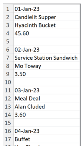
Look familiar? This causes analysts significant grief as they try not to undertake some repetitive, manual procedure to put this data into a more usable format — see the screenshot “Usable format”.
Usable format
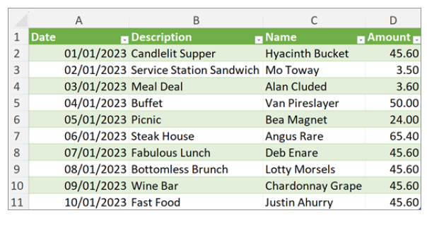
Now wouldn’t it be something if you could automate and produce this in seconds? You can do this with Power Query/Get & Transform (it is called the latter in Excel until you open the editor; it then reverts to its old name).
In Office 365, highlight the original data and go to the Data tab of the Ribbon; click From Table/Range in the Get & Transform Data group (see the screenshot “Selecting From Table/Range”).
Selecting From Table/Range
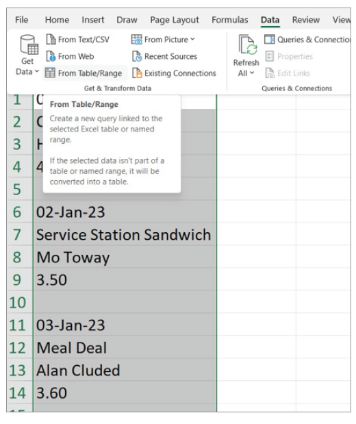
(Depending upon your version of Excel, your interface may look slightly different.)
Having confirmed your Table area and indicated that there are no headings, this opens the Power Query Editor, which displays the complete list highlighted. You can delete the Changed Type step (which decides whether the field contains text, numbers, dates, etc.) by using the cross next to it. Since the column has mixed data types, the types can be defined later when you have split them up. (See the downloadable screenshot “Deleting the Changed Type Step”.)
Going to the Add Column tab of the Ribbon, select From 0 in the drop-down list of Index Column (see the downloadable screenshot “Adding Column From 0”).
This creates a sequential counter in a second column starting from zero [0] (see the downloadable screenshot “Creating a Sequential Counter”).
Do you see how the steps are being detailed in the APPLIED STEPS section of the Query Editor (in the right-hand pane)? Power Query is recording the steps, so you only need to make these transformations once and use them at your leisure thereafter.
Now, highlight the Index column and select Divide (Integer) from the Standard drop-down box on the Add Column tab of the Ribbon — see the downloadable screenshot “Selecting Divide (Integer)”.
This allows you to add another column where you can divide the index by a number and it returns just the whole number, eg, 28 divided by 8 is 3 remainder 4, so would return a value of 3. The number we want, though, is the index number for the first row of the second block of data (here, this is 5) — see the downloadable screenshot “Entering a Number in the Integer-Divide Dialogue Box”.
Once you click OK, a second column is added — see the downloadable screenshot “Inserting the Integer-Division Column”.
It’s time for me to explain. The third column, Integer-Division, is going to represent the row number for the data (so all the rows with the same Integer-Division number will end up on the same row of the final table to be generated). The second column, Index, was needed to generate it. Now, I need to use Index for something else.
Highlight the Index column again and select Modulo from the Standard drop-down box on the Transform tab of the Ribbon. Again, we use the number five [5] for the same reasons as earlier (see the downloadable screenshot “Selecting Modulo from the Standard Drop-Down Box”).
Clicking OK creates the recurring sequence 0, 1, 2, 3, and 4 in the Index Field (see the downloadable screenshot “Creating Recurring Sequence in the Index Field”).
Can you see where this is going? If I use the third column (Integer-Division) as my row number and Index as my column number, I have my coordinates for each value in Column1. All I need to do is select the Index column and click on Pivot Column on the Transform tab of the Ribbon (see the downloadable screenshot “Selecting Index Column and Clicking on Pivot Column”.)
From the resulting dialog box, select Column1 for the values. That’s not enough, though, as we will only get a count of the items. From the Advanced options box, select Don’t Aggregate from the Aggregate Value Function (this allows the value to be displayed when it is text) — see the downloadable screenshot “Selecting Column1 and Don’t Aggregate”.
Clicking OK makes everything come into sharp focus (see the screenshot “Clicking OK”.)
Clicking OK

To tidy up, remove the first and last columns and rename each field (right-clicking on each column allows access to these options). Then use CTRL + A to select all the columns and use Detect Data Type on the Transform tab to select the appropriate data types using Power Query’s algorithms (see the screenshot “Tidying Up in Power Query Editor”.)
Tidying up in Power Query Editor
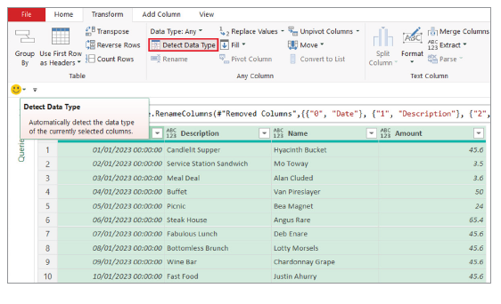
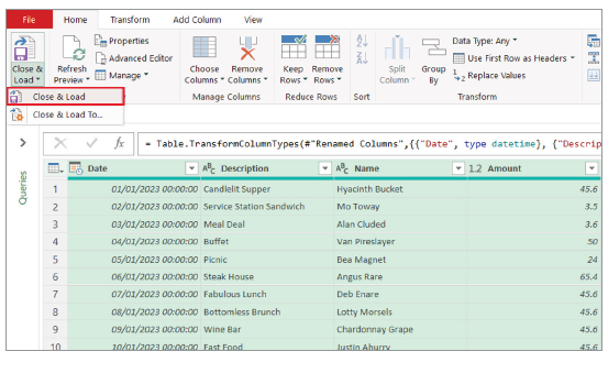
Once finished, from the Home tab, simply select Close & Load (see the screenshot “Select Close & Load”.)
Select Close & Load
And there you have it! (See the screenshot “Final Table”.)
Final table
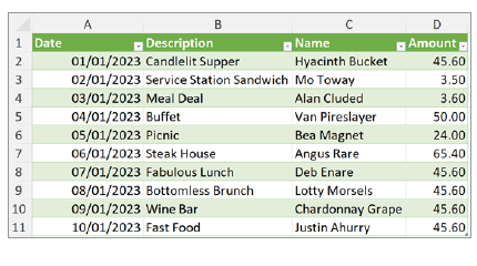
The great thing about having performed this using Power Query is that if the table changes, the final table can be refreshed with just a click (of the Refresh button).
Liam Bastick, FCMA, CGMA, FCA, is director of SumProduct, a global consultancy specialising in Excel training. He is also an Excel MVP (as appointed by Microsoft) and author of Introduction to Financial Modelling and Continuing Financial Modelling. Send ideas for future Excel-related articles to him at liam.bastick@sumproduct.com. To comment on this article or to suggest an idea for another article, contact Oliver Rowe at Oliver.Rowe@aicpa-cima.com.


