I thought it was time to examine Excel’s features and updates specifically for images. There are several options, including how you can now obtain table data from pictures and how images may also be inserted into spreadsheet cells. There is also an IMAGE function for formatting pictures inserted in cells, and, believe it or not, you may now insert pictures into PivotTables, too.
Let’s take a look — see also the example Excel file.
Get Data From Picture
Available in Excel for Microsoft 365, Excel is now able to extract data from pictures. Users may extract data tables from photos or screenshots. The option can be found in the Data tab, in Get & Transform Data -> From Picture using pictures either from a file or already copied to the Clipboard (see the screenshot “Extracting Data From Picture”).

This means it is now quite easy to take screenshots and import data into Excel. For example, see the screenshot “Sample Dataset” for a sample fictional dataset that our company SumProduct uses for modelling.

After I take a screenshot of it, I can then click the option Picture From Clipboard, described above, and Excel will start to load and analyse the picture.
Upon completion, the Data from Picture pane produces a data preview and highlights the values that need to be further verified by the user — see the screenshot “Data Preview — for Verification”.

You may then confirm or amend the highlighted cells (shaded in light red) and input the data into Excel as a range. As a tip, it’s always advisable to crop the image and only include the target area. In this case, you can see that Excel has detected a lot of unnecessary information. We only wanted the table. Therefore, allow me to repeat the exercise but this time crop the screenshot (in this example, I am simply using the Windows Snipping Tool) — see the screenshot “Cropping to Include Only the Target Area”.
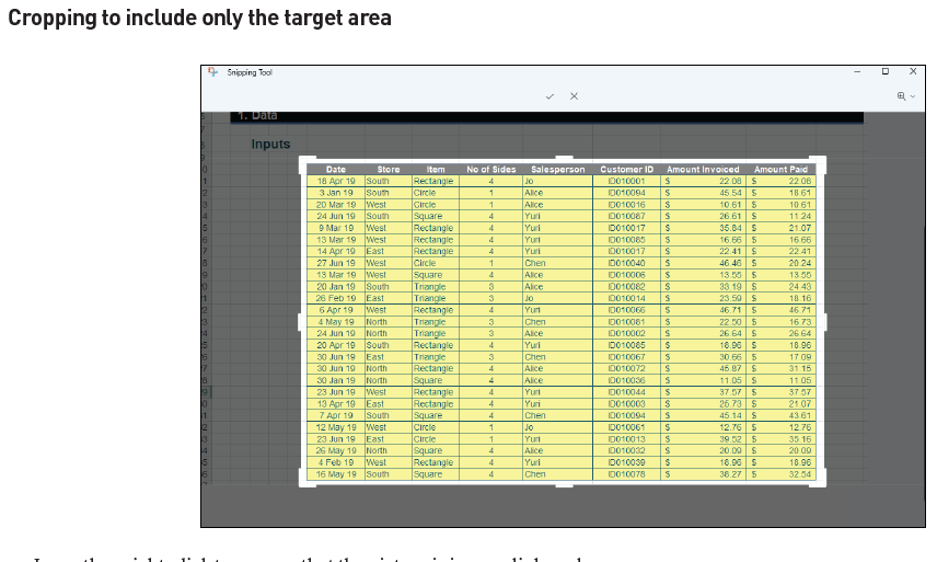
I may then right-click to copy so that the picture is in our clipboard.
I then use Picture From Clipboard again to import the picture into Excel — see the screenshot “Data Preview — Revised”.
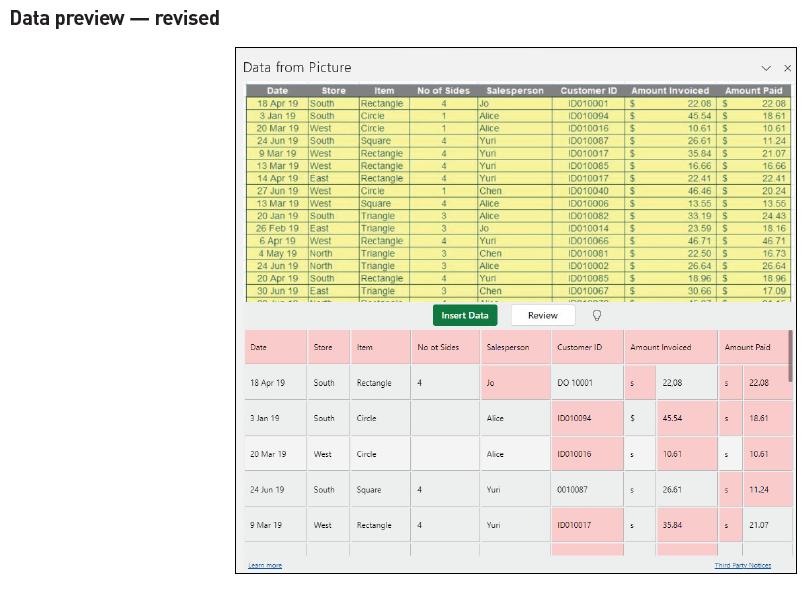
You will notice that Excel’s image recognition is not yet perfect, but, quite frankly, it is a lot better than several other options I have tried in the past.
In particular, the Customer ID column requires further assistance, even cells that aren’t shaded red. I can try to review and amend as much as possible with the Data from Picture pane before inserting the data and making any manual corrections in Excel itself.
One useful feature of the Data from Picture pane is that it zooms its window to the relevant area when you click on a detected cell (hence the lower resolution in the source image in the screenshot “Zooming to Relevant Area From Detected Cell”), making it very easy for the user to cross-reference.
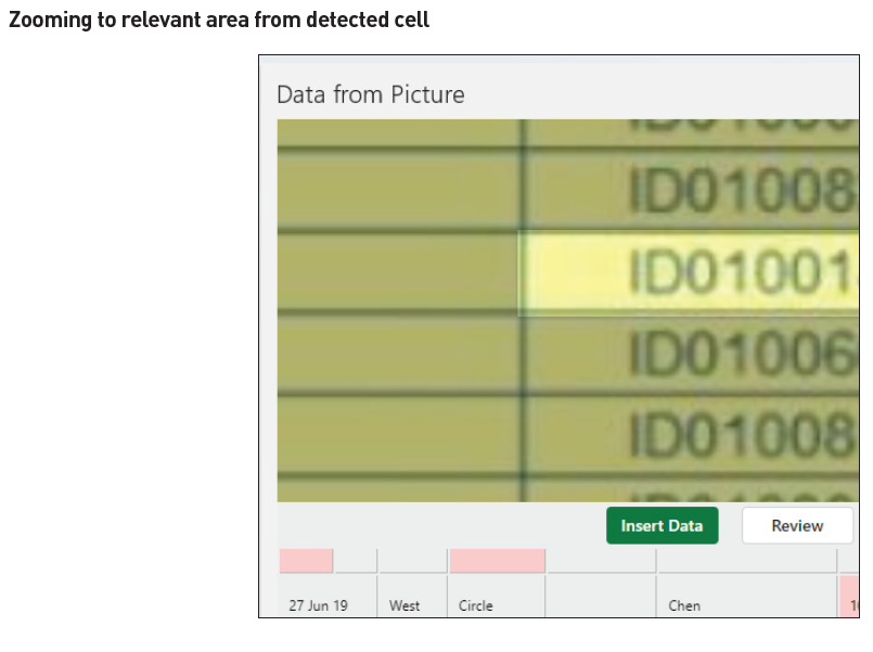
Some text inputs (eg, ID numbers), once incorrectly entered as numbers, might be quite hard to guess and amend without returning time and again to the source data.
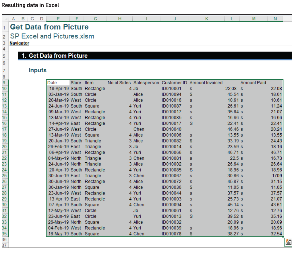
Albeit far from perfect, in this illustration at least, Excel still does an adequate job picking up much of the detailed information, such as Date, Store, Item, Salesperson, Amount Invoiced, and Amount Paid. That reduces the manual work required. (See the screenshot “Resulting Data in Excel”.)
You may also insert data from a graphic file, which provides more flexibility. For example, you can try to scan printed materials or even hand-drawn tables. Here is a list of graphic file types that may be inserted presently in Microsoft Office documents (correct as of the time of this writing):
BMP, EMF, EMZ, EPS, Fpix, FPX, GIF, JPEG, JFIF, JPEG-2000, PDF, PICT, PCT, PNG, PNTG, PSD, QTIF, SGI, TGA, TPIC, TIFF, TIF, WMF, WMZ.
Data from Picture does have some limitations: Excel scans numerical values more accurately and less so for text values or where there may be a combination of the two (eg, ID numbers). In addition, Excel scans printing-font tables reasonably well (either from screenshots or photos), but it struggles with handwritten data.
Furthermore, my team has noted that Excel’s Data from Picture feature would be useful for getting data from scanned PDF documents (as there are no searchable or selectable text but only images), especially where Power Query (Get & Transform) was unable to extract the data. In this instance, you can use this feature to extract data from these scanned PDF files, rather than having to manually read and input the data.
Insert Picture in Cell
Another new feature of Excel is that you are now able to insert pictures in cells. This should not be confused with the legacy method of placing pictures on top of spreadsheet cells.
Placing a picture on top of spreadsheet cells is the default behaviour of Excel. Although Excel no longer allows pasting or drag-and-dropping a graphic file, pasting an image from the clipboard still puts it on top of the cells, ie, as a Picture over Cells. (You may also use the Ribbon option: Go to the Insert tab and then select Pictures -> Place over Cells, where you may browse for a graphic file and other sources such as Stock Images in Excel or Online Pictures.
To return to the new feature: There are four ways to insert a picture into a cell:
1. Insert Picture in Cell from the Excel Ribbon;
2. Paste Picture in Cell from the Clipboard;
3. Switch from Picture over Cells to Picture in Cell; and
4. With the IMAGE function, using a web URL path.
The first option is to insert a picture into a cell from the Ribbon. Going to Insert -> Pictures -> Place in Cell provides you with several options to insert a picture into the active cell. There is the common option of browsing for a local graphic file, but there are also a few more different sources of pictures, too (see the screenshot “Sources of Pictures to Insert”).
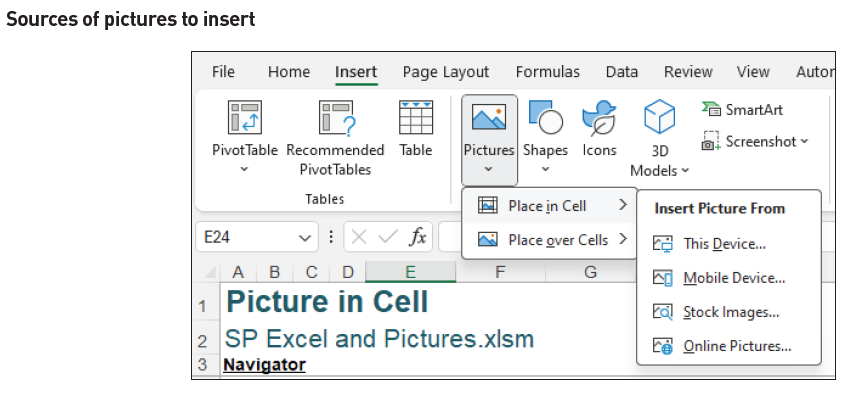
For example, Stock Images… offers a rich collection of different types and different themes of pictures.
You may also paste a picture into a cell from the Clipboard. Of course, you first need to have an image in the Clipboard. In the example of getting an online image, you may right-click to Copy image and then right-click on the cell to insert, using the Paste Picture in Cell option (last icon under Paste Options). (See the screenshot “Pasting a Picture Into a Cell From the Clipboard”.)

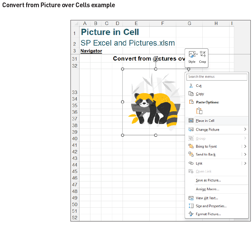
The third way identified to put a Picture in Cell is to convert from a Picture over Cells. Here, I have prepared a racoon image floating over spreadsheet cells. When I right-click on the racoon, you will see the option Place in Cell — see the screenshot “Convert From Picture Over Cells Example”.
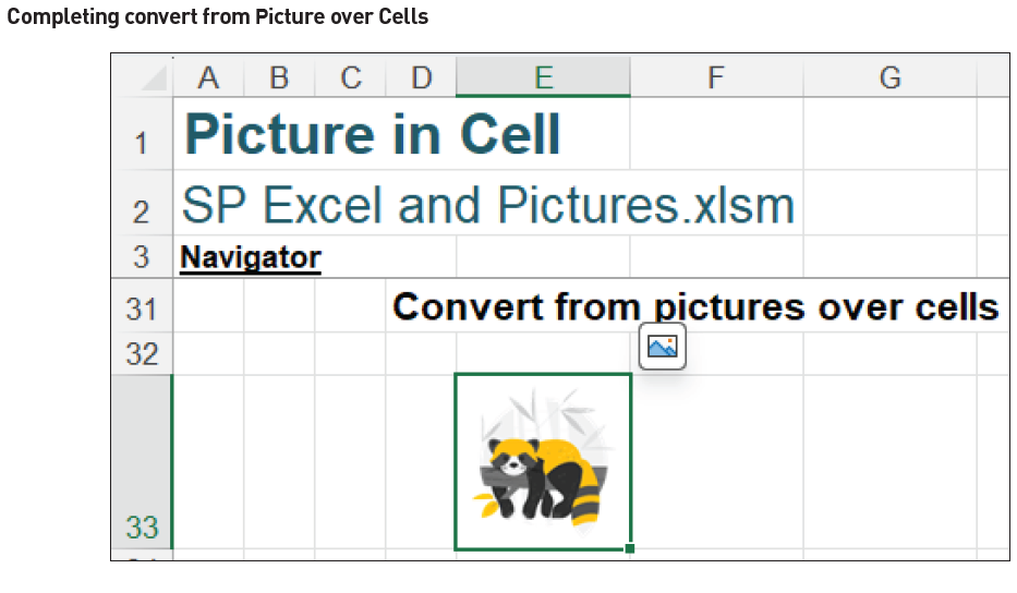
Using this option places the racoon into the top-left cell of the region that it had been floating over (see the screenshot “Completing Convert From Picture Over Cells”).
The final step, and probably the most technical method to insert a Picture in Cell, is to use the IMAGE function. This function offers different sizing options and also allows you to input descriptive alternative text. However, I will save this for later when I discuss the IMAGE function and its applications.
Picture in Cell has fewer formatting options compared to the legacy Picture over Cells. Let me demonstrate. A Picture in Cell has a fixed aspect ratio (height-to-width ratio), and it cannot be changed by resizing the cell it resides in — see the screenshots “Fixed Aspect Ratio Examples”.
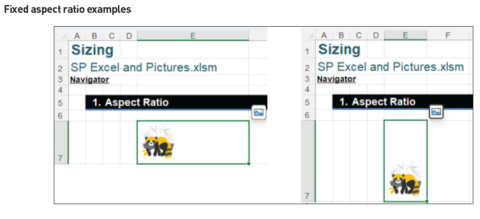
The only exception is when using an IMAGE function to create a Picture in Cell and changing the function arguments (more anon).
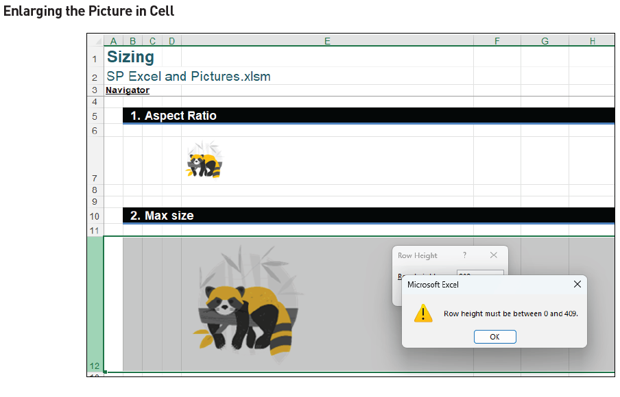
The size of a Picture in Cell is also limited by the cell containing it. You may increase the cell’s height and width to enlarge the picture inside, but Excel has a maximum row height of 409 cm and a maximum column width of 255 characters — so that is as large as the picture can be (see the screenshot “Enlarging the Picture in Cell”).
One way to work around this limitation (if you really want to have an enormous image in a single cell, that is) is to merge cells vertically and expand the relevant rows (see the screenshot “Working Around Picture in Cell Size Limitation”).
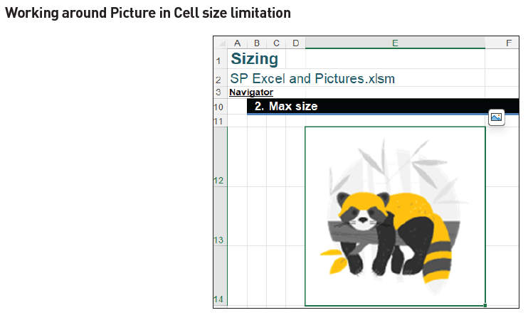
You can further expand rows 12, 13, and 14 to a height of 409 cm, and this will work around the restriction.
When Picture in Cell is being resized, it does not change the workbook size. If we consider our racoon above that is now occupying three rows, the Excel workbook has a present file size of 395 kilobytes:

If I revert to a compact unmerged square cell (48cm×8.43char) (see the screenshot “Reverting to Compact Unmerged Square Cell”),
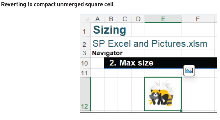
the workbook remains 395 kilobytes:

Another formatting option to consider is that you cannot edit the colours of a Picture in Cell, whereas this is an option for the legacy Picture over Cells. However, I may still fill colours in the cell containing the image.
When pictures are inserted into cells, Excel handles them much like values (eg, numbers or text). You may copy and paste a Picture in Cell, and you may even use it in a formula to produce formulaic graphical outputs.
Here, I have prepared an example with the 12 Chinese Zodiac animals (see the screenshot “Chinese Zodiac Animals”).
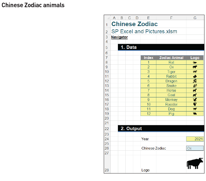
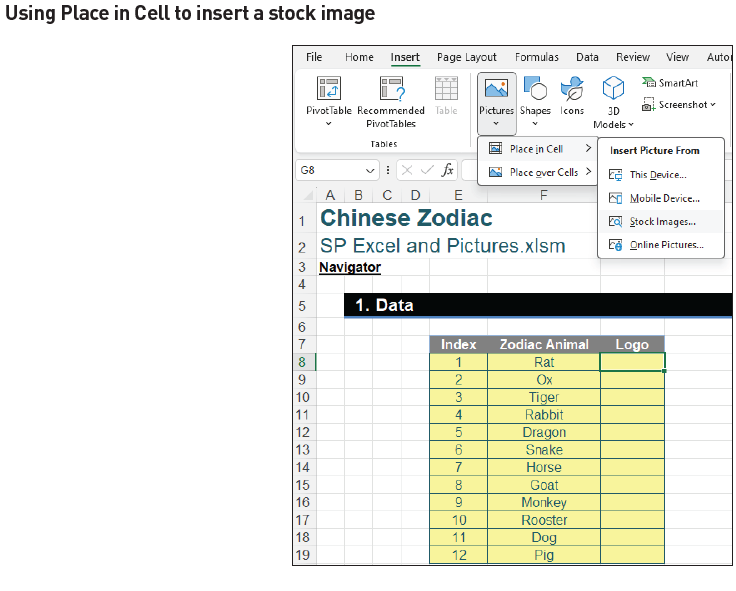
I built the input images from Excel’s Stock Images… . To demonstrate, let’s take the animal Rat as an example. Select the cell where the image should be inserted (here, cell G8), and then go to the Insert tab and Pictures -> Place in Cell -> Stock Images… . (See the screenshot “Using Place in Cell to Insert a Stock Image”.)
This will open up the Search window (see the screenshot “Search Window”).
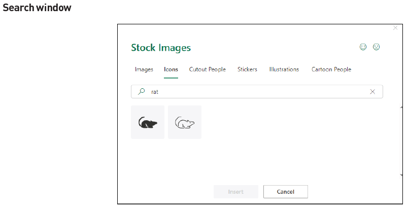
I then searched and found a rat icon and inserted it. Repeating this exercise for all 12 animals completed the input table, with 12 pictures in cells for the 12 Chinese Zodiac animals.
I also inserted the input as a Table (CTRL+T), called ZodiacTable, for formula transparency. In our output, I may use XLOOKUP to return the Chinese Zodiac animal for a certain year and, more importantly, the corresponding logo (see the screenshot “Using XLOOKUP and a MOD Formula”).
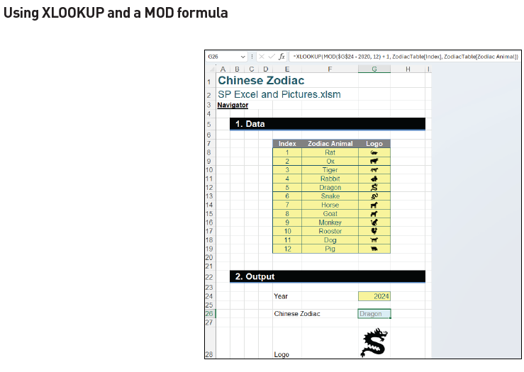
=XLOOKUP(MOD($G$24 – 2020, 12) + 1, ZodiacTable[Index], ZodiacTable[Zodiac Animal])
Here, I have used a MOD formula to calculate which zodiac animal a certain year relates to:
MOD($G$24 – 2020, 12) + 1
I have used the year 2020 as my basis as I know it is a Year of the Rat, the first in the cycle. The MOD function will take the value in cell G24 (anchored), subtract 2020 from it, and divide the result by 12 (the number of different years in the cycle). This will provide a remainder between zero [0] and 11 inclusive. Adding one [1] results in a value from 1 to 12 instead. Wrapping this MOD expression in an XLOOKUP calculation, I may find the animal for a year:
=XLOOKUP(MOD($G$24 – 2020, 12) + 1, ZodiacTable[Index], ZodiacTable[Zodiac Animal])
Then I may make a similar formula to return a Picture in Cell, ie, the relevant logo:
=XLOOKUP(MOD($G$24 -2020, 12) + 1, ZodiacTable[Index], ZodiacTable[Logo])
Now I have a dynamic Picture in Cell indicating the Zodiac logo of a year! (See the screenshots “Examples Indicating a Year’s Logo”.)
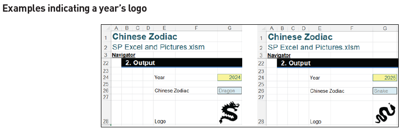
IMAGE function
Now, let’s turn our attention to the aforementioned IMAGE function. This function inserts images into cells from a source location along with alternative text. It has the following syntax:
=IMAGE(source, [alt_text], [sizing], [height], [width])
The arguments are as follows:
source is required and represents the URL path of the image file, using an https protocol (it should be noted that supported file formats include BMP, JPG, JPEG, GIF, TIFF, PNG, ICO, and WEBP). Upon modifying as required, cell references within the workbook appear to be recognised, too.
alt_text is the first optional argument. This is the alternative text that describes the image (for accessibility purposes).
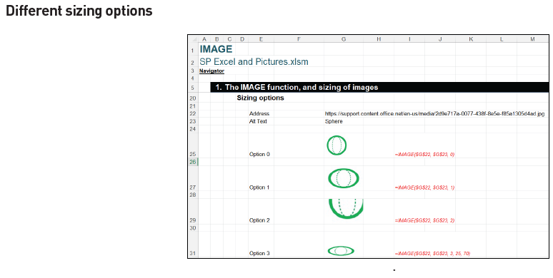
sizing is also an optional parameter and specifies the image dimensions. There are several possible values:
- 0: Fit the image in the cell and maintain its aspect ratio (default).
- 1: Fill the cell with the image and ignore its aspect ratio.
- 2: Maintain the original image size, which may exceed the cell boundary.
- 3: Customise the image size by using the height and width arguments (see below).
height and width are optional arguments. These define the height and width, respectively, of the image only when using sizing option 3 (see above).
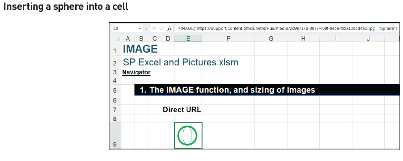
Let’s look at a few examples. You can insert a sphere into a cell with the formula:
=IMAGE(“https://support.content.office.net/en-us/media/2d9e717a-0077-438f-8e5e-f85a1305d4ad.jpg”, “Sphere”)
(See the screenshot “Inserting a Sphere Into a Cell”.)
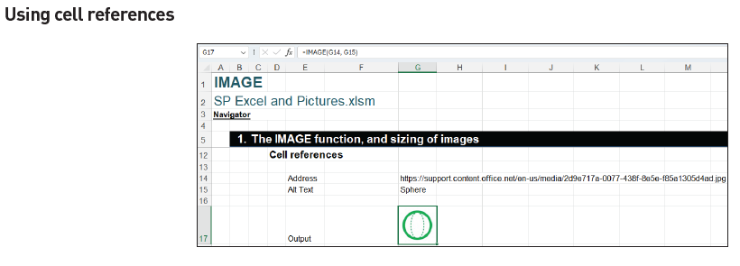
We could also use cell references to be flexible and transparent — see the screenshot “Using Cell References”.
As for the different sizing options, the default option, zero [0], fits the image in the cell and maintains its aspect ratio. Option 1 fills the cell with the image; option 2 maintains the original image size; and option 3 customises the image size by using the height and width arguments (see the screenshot “Different Sizing Options”).
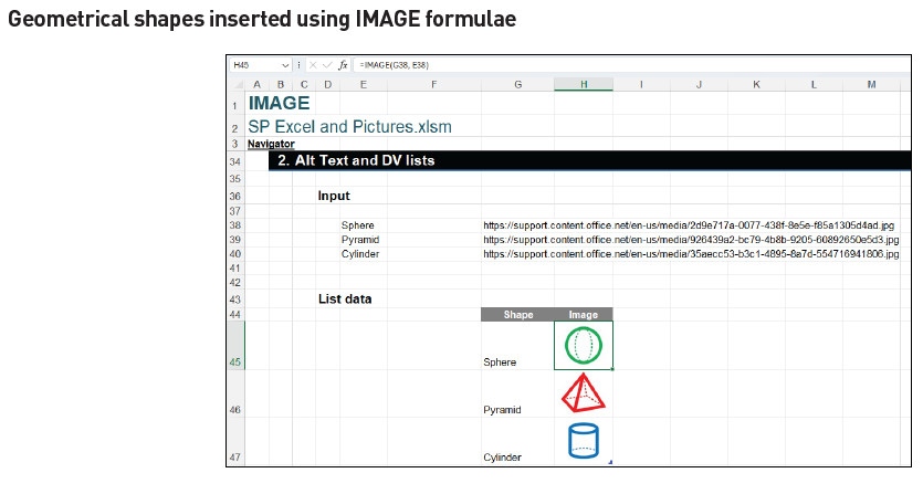
Moreover, we want to show you some creative graphics tricks for Data Validation (ALT+D+L) lists, using the IMAGE function together with alternative text. I have listed a few geometrical shapes from Microsoft and used IMAGE formulae to insert them into cells and then created a Table (CTRL+T) called Dvimage (see the screenshot “Geometrical Shapes Inserted Using IMAGE Formulae”).
Then, I have created a Data Validation dropdown list with the column of images using Data -> Data Validation -> Data Validation… (see the screenshot “Creating Data Validation Dropdown List”).

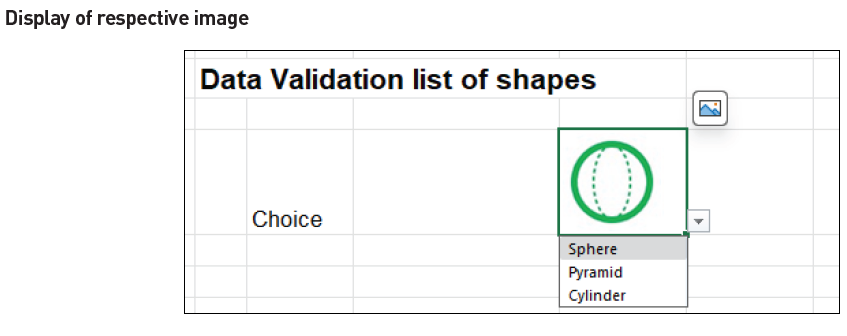
By generating this dropdown list, you will see that the descriptive alternative text is used for the list but, once selected, displays the respective image instead — see the screenshot “Display of Respective Image”.
Display pictures in PivotTables
We can even use pictures inserted in cells for PivotTables.
For example, we can use country flags for a sales dataset. Let’s consider a sample sales dataset from Microsoft — see the example Excel file.
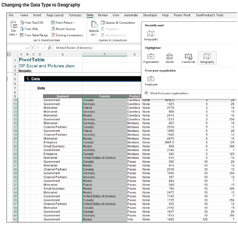
In the sales dataset, we can change Data Type of the Country column to Geography (see the screenshot “Changing the Data Type to Geography”).
Then, I can access other information from a Geography type (including flag images). We insert the above as a Table (CTRL+T) called PivotData. I insert a column Flag and use the dot operator (.) To get the flag images of the countries (see the screenshot “Inserting a Column Flag”).
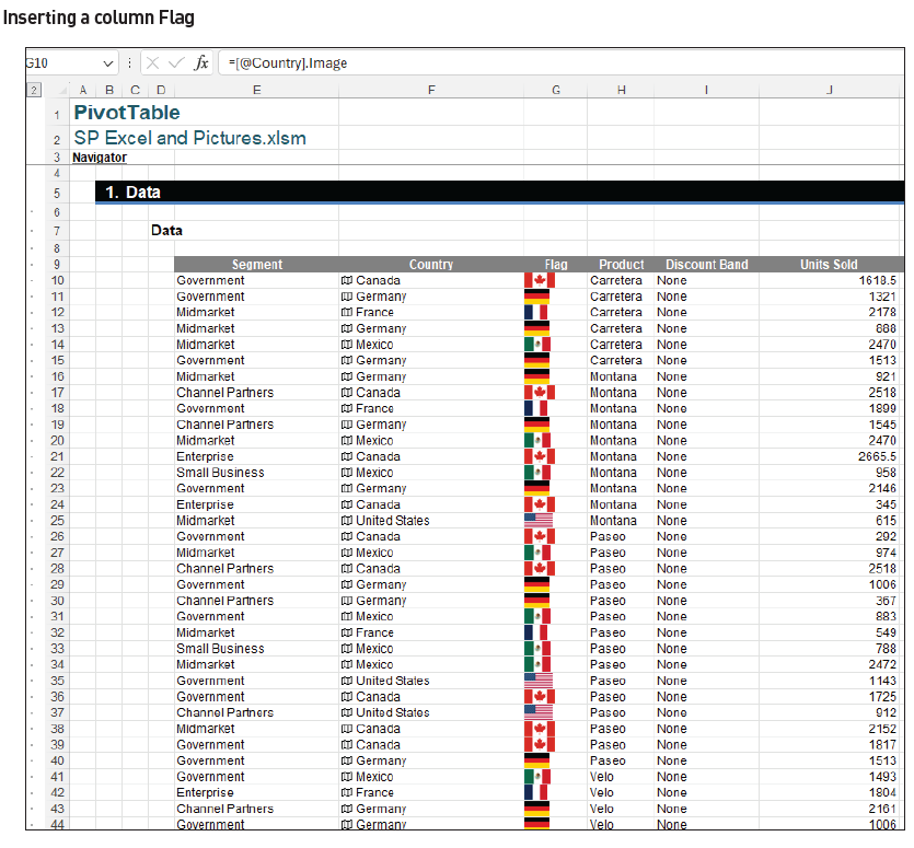
=[@Country].Image
Then we are able to insert a PivotTable and use images from the column Flag, in either row or column fields — see the screenshots “Using Flags in PivotTable columns” and “Using Flags in PivotTable Rows”.
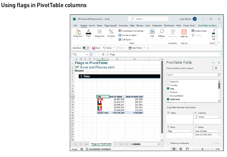
We can use inserted images as row and column fields. However, filters and slicers are not that sophisticated — yet!

Do remember that this is a feature for pictures inserted into cells only. It is not for the legacy floating images over cells. You should also note that presently we cannot load and process inserted images into Power Query.
Word to the wise
Hopefully, this has been a useful discussion for you, providing plenty of ideas for future reports, charts, dashboards, and other visualisations in Excel. Presently, much of this only works in Excel 365 — and then sometimes only in certain versions.
Please don’t let that put you off. The future is coming, and every picture you add can potentially replace some reports.
Liam Bastick, FCMA, CGMA, FCA, is director of SumProduct, a global consultancy specialising in Excel training. He is also an Excel MVP (as appointed by Microsoft) and author of Introduction to Financial Modelling and Continuing Financial Modelling. Send ideas for future Excel-related articles to him at liam.bastick@sumproduct.com. To comment on this article or to suggest an idea for another article, contact Oliver Rowe at Oliver.Rowe@aicpa-cima.com.


