Top 5 Excel functions you might not know

So, it went something like this…

Editor: “I’d like you to write an article about the top five Excel functions accountants need to know.”

Me: “Hmm, the most common ones include SUM, IF, SUMIF, SUMIFS, or SUMPRODUCT; VLOOKUP (yuck!) or INDEX(MATCH); OFFSET; MOD; and one of MAX and MIN — that will be a riveting read …”

Editor: “How about five powerful functions they should be using?”

Me: “That might be some of the new functions such as XLOOKUP, SORT, UNIQUE, FILTER, and SEQUENCE … I have written a lot about these recently, and besides, those are available only on Office 365, not Excel 2019, or Excel 2013, or Excel 2010, or …”

Editor: “OK, I get the point. How about the top five functions you should be using that have been around for a while and are accessible to standard Excel users?”

Me: “Good idea!”

There you have it. Dear reader, I present the top five functions that are available right now (and have been for some time) that you might not be using.

These are not necessarily your usual suspects, in alphabetical order.

1. AGGREGATE

You could argue this is the most complicated Excel function of all time. AGGREGATE began life in Excel 2010. For those who desire greater sesquipedalian loquaciousness (look it up), its syntax may give even more comfort, as it has two forms:

1. Reference: AGGREGATE(function_number, options, ref1, [ref2], …).

2. Array: AGGREGATE(function_number, options, array, [optional_argument]), where:

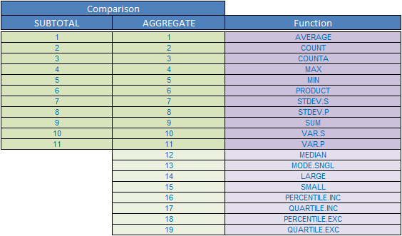
• function_number denotes the function that you wish to use. Similar to the SUBTOTAL function, function_number allocates integer values to various Excel functions:

• options specifies which values may be ignored when applying the chosen function to the range. If the options parameter is omitted, the AGGREGATE function assumes that options is set to zero (0). The options argument can take any of the following values:

• ref1 is the first numeric argument for the function when using the Reference syntax.
• ref2, ... is optional. Numerical arguments may number two through 253 for the function when using the Reference syntax.
• array is an array, array formula, or reference to a range of cells when using the Array syntax.
• optional_argument is a second argument required if using the LARGE, SMALL, PERCENTILE.INC, QUARTILE.INC, PERCENTILE.EXC, or QUARTILE.EXC function when using the Array syntax:

As already mentioned, AGGREGATE is analogous to an extension of the SUBTOTAL function insofar that it uses the same function_number arguments, adding another eight. SUBTOTAL allows you to use the 11 functions including/excluding hidden rows, which results in 22 combinations. However, AGGREGATE goes further and takes the 19 functions and allows for eight alternatives for each, which results in 152 combinations — and that’s not even considering the Reference or Array syntax approaches!

It just all sounds, well, tremendously complicated. This example Excel file helps demystify.

In practice, it’s not that bad. This is because, since this function was created, screen tips will appear as you type in order to nudge you in the right direction. For example, let’s say you wanted the third-largest number in the following list:

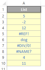
From inspection, the third-largest value is the amount in cell A2 (the value “5”), but if you use the usual formula for this =LARGE(A2:A10,3), you will get the value #REF!, as this is the first error that Excel comes across as it works down the list.

This is where you can use AGGREGATE to ignore these errors. If you type in =AGGREGATE(, you will get the following screen tip scroll list:

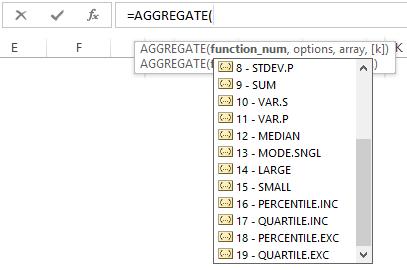
By typing “14” or selecting “14 - LARGE” from the pop-up list, you now know you are on the right track. After typing a comma, Excel then continues to help you:

Again, by either typing a number or pointing and clicking, an appropriate choice may be made. I want to ignore errors, so I need to choose “2”, “3”, “6”, or “7”, depending upon what else should be ignored. I will choose “6” — ignore error values only and then type another comma so that the screen tips keep coming thick and fast:

Now, Excel is seeking the references for evaluation. It appears to be possible that this can be in the form of a list (the array) or else discrete cell references and/or values. In this example, I will enter the range and type another comma:

Now, Excel appears to be looking for the other argument for LARGE() or else another reference. This is not correct. The screen tip does not update automatically. The syntax required is now just as it would be if we had typed in the underlying function, ie, =LARGE(array, k). In this instance, this syntax always requires the fourth value to be k, the integer denoting the kth-largest item in the list.

In this example, I will just type the value “3” and close brackets. Therefore, we arrive at the following formula:

=AGGREGATE(14,6,A2:A10,3)

which generates the correct answer “5”. The formula might look counterintuitive, but Excel has helped us every step of the way. As my oft-misquoted English teacher always used to say, practice makes perfect. Please see the attached Excel file for more examples.

To summarise, like SUBTOTAL, the AGGREGATE function is designed for columns of data (vertical ranges), not for rows of data (horizontal ranges). For example, when you subtotal a horizontal range using option 1, such as AGGREGATE(1, 1, ref1), hiding a column does not affect the aggregate sum value, although hiding a row in vertical range does affect the aggregate.

If a second ref argument is required but not provided, AGGREGATE returns a #VALUE! error.

If one or more of the references are three-dimensional references, AGGREGATE, like above, returns a #VALUE! error.

2. EOMONTH

Dates are very important to accountants and should not just be hard-coded into a spreadsheet. We often need them to vary. We tend to work with month end dates, and this is where this function becomes invaluable. We usually run across one of the top rows in an Excel worksheet as part of a time series analysis:

In this example, a monthly model has been constructed starting in July 2020. The dates in cells J5 onwards are formatted to show only the month and year. However, if I were to format the cell as General instead (Ctrl+1), note that the Sample (circled in red) would be displayed as follows:

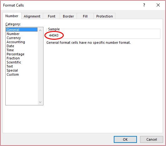
In other words, 31 July 2020 is no more than a number: 44,043. Microsoft Excel for Windows supports what is called the 1900 date system. This means that 1 January 1900 is considered to be day 1 by Excel, 2 January 1900 is day 2, and so on.

Clearly, dates are not as easy to manipulate as you might think. Extracting the day, month, or even the year from any given date is not straightforward because the date is really a number known as a serial number.

Extracting a day, month, or year requires using the following three functions:

• DAY(serial_number) gives the day in the date (for example, DAY(31-Jul-20) = 31).

• MONTH(serial_number) gives the month in the date (for example, MONTH(31-Jul-20) = 7).

• YEAR(serial_number) gives the year in the date (for example, YEAR(31-Jul-20) = 2020).

It is just as awkward the other way around. If the day, month, and year are already known, the date can be calculated using the following function:

DATE(year, month, day) (for example, DATE(2020,7,32) = 1 August 2020, etc.).

Did you catch the function calculates the 32nd day of July as 1 August? Since dates are nothing more than serial numbers, they behave just like formatted numbers in Excel, for example, 31-Jul-20 + 128 = 6-Dec-2020.

This is all great, but time series still cause us problems. If we want to have the month end date in each column, we cannot simply take the previous month’s date and add a constant to it, since the number of days in a month varies. Fortunately, this is where EOMONTH comes in:

EOMONTH(specified_date, number_of_months)

The “End Of Month” (EOMONTH) function therefore calculates the end of the month as the number_of_months after the specified_date. For example:

• EOMONTH(31-Jul-20,0) = 31-Jul-20.

• EOMONTH(3-Apr-05,2) = 30-Jun-05.

• EOMONTH(29-Feb-08,-12) = 28-Feb-07.

Although the examples use typed-in dates, for it to work in Excel, it is best to have the specified_date either as a cell reference to a date or else use the DATE function to ensure that Excel understands it is a date (otherwise the formula may calculate it as #VALUE!).

In some instances (for example, appraisal of large-scale capital infrastructure projects), the dates may need to be for the same day of the month (for example, the 15th) rather than for the month end. A function similar to EOMONTH, EDATE can be used instead:

EDATE(specified_date, number_of_months).

The “Equivalent day” (EDATE) function therefore calculates the date that is the indicated number_of_months before or after the specified_date. For example:

• EDATE(15-Jul-20,2) = 15-Sep-20.
• EDATE(3-Apr-05,-2) = 3-Feb-05.
• EDATE(29-Feb-28,-12) = 28-Feb-27.

If an equivalent date cannot be found (as in the last example), month end is used instead.

3. FORMULATEXT

New to Excel 2013, this is one of the most used functions by my team. It’s a really useful tool for documenting formulas, as FORMULATEXT returns a formula as a text string. People have been writing User-Defined Functions (UDFs) for years to replicate this functionality.

In fact, if you have ever downloaded one of my example workbooks, the chances are you have analysed a formula described using the FORMULATEXT function:

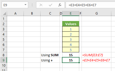
The expressions in cells G8 and G9 (above) are both provided by the FORMULATEXT function. For example, the formula in cell G8 is:

=FORMULATEXT(E8).

The FORMULATEXT function employs the following syntax to operate:

FORMULATEXT(reference)

It has the following argument:

• reference: This is required and represents a cell or a reference to a range of cells.

It should be further noted that:

• The FORMULATEXT function returns what is displayed in the formula bar if you select the referenced cell.
• The reference argument can be to another worksheet or workbook.
• If the reference argument is to another workbook that is not open, FORMULATEXT returns the #N/A error.
• If the reference argument is to an entire row or column, or to a range or defined name containing more than one cell, FORMULATEXT returns the value in the upper leftmost cell of the row, column, or range.
• In the following cases, FORMULATEXT returns the #N/A error:
  • The cell used as the reference argument does not contain a formula.
  • The formula in the cell is longer than 8,192 characters.
  • The formula cannot be displayed in the worksheet, for example, due to worksheet protection.
  • An external workbook that contains the formula is not open in Excel.
• Invalid data types used as inputs will produce the #VALUE! error.
• Entering a reference to the cell in which you are entering the function as the argument will not result in a circular reference warning. FORMULATEXT will successfully return the formula as text in the cell.

I love this example:

4. N

I love functions I can spell. The N function returns a value converted to a number. It has only one argument:

N(value)

The value argument is required and represents the value you want converted. N converts values on the following basis:

Usually, you don’t need to use the N function in a formula because Excel automatically converts values as necessary. Microsoft states that this function is provided for compatibility with other spreadsheet programs. However, I disagree: I use this function all the time. Let me explain.

Counters are often used in financial modelling, eg:

It’s not a good idea to type these numbers in and/or use AutoFill. This is because if an end user wishes to extend the sequence, they might take the first cell (D2) and drag it across. Unfortunately, in this scenario, you would get a sequence of 1’s, viz.

Oops. Therefore, we should use a formula in cell D2 such as =C2+1:

That’s all well and good, until someone types something in cell C2:

The problem is cell C2 now contains text, and you cannot add one (1) to text. However, you can add N to the formula:

The N function ignores the text in cell C2. That’s exactly what we require. I use counters in my financial models all the time — and, therefore, I use the N function all the time, too.

5. TEXTJOIN

The TEXTJOIN function combines the text from multiple ranges and/or text strings and includes a delimiter to be specified between each text value to be combined. If the delimiter is an empty text string, this function will effectively concatenate the ranges similar to the CONCAT function. Its syntax is:

TEXTJOIN(delimiter, ignore_empty, text1, [text2], …)

where:

• delimiter is a text string (which may be empty) with characters contained within inverted commas (double quotes). If a number is supplied, it will be treated as text.

• ignore_empty ignores empty cells if TRUE or the argument is unspecified (ie, is blank).

• text1 is a text item to be joined.

• text2 (onwards) are additional items to be joined up to a maximum of 252 arguments. If the resulting string contains more than 32,767 characters, TEXTJOIN returns the #VALUE! error.

TEXTJOIN is more powerful than CONCAT. To highlight this, consider the following examples:

Here, in the formulas on rows 53 and 54, empty cells in a contiguous range may be ignored, and delimiters only need to be specified once. It’s a great way to create lists for reporting, for example.

— Liam Bastick, FCMA, CGMA, FCA, is director of SumProduct, a global consultancy specialising in Excel training. He is also an Excel MVP (as appointed by Microsoft) and author of Introduction to Financial Modelling. Send ideas for future Excel-related articles to him at liam.bastick@sumproduct.com. To comment on this article or to suggest an idea for another article, contact Jeff Drew, an FM magazine senior editor, at Jeff.Drew@aicpa-cima.com.