Financial modelling plays a vital role helping businesses make financial decisions by forecasting the future results based upon historical data and current assumptions. However, as data evolves and new information emerges and is gleaned, financial models must adapt and integrate accordingly, ie, link appropriately while reporting flexibly and consistently.
This is where scalable financial models come into play by offering the end user the ability to add or modify inputs — for example, extending the number of periods, revising product types, and considering newly acquired businesses or divisions.
Let’s consider how to design an Excel financial model with the necessary flexibility and scalability borne in mind.
Definition
A scalable financial model is designed to accommodate growth in multiple dimensions without major structural changes. It might use Tables, dynamic array formulas, or even create new sheets to achieve the scalability required. A new line of business, a new product, or even a new entity may be added to the model with minimal adjustments.
Besides using these tools, we can also design scalable models in what is known as a “modular format” with many reusable components, designed to be later duplicated or copied and pasted to create new sections. It is important to consider the designs required for scalability in the model in advance, so that model consistency, robustness, flexibility, and transparency (CRaFT) are maintained.
Here are six ways to introduce flexibility into an Excel financial model to allow scaling up without structural changes.
1. Dynamic arrays
One option is to adopt dynamic arrays. A dynamic array is a feature in Excel that enables a formula to automatically expand or contract (a feature known as “spilling”). A particularly notable dynamic array function is SEQUENCE, which may be used in conjunction with INDIRECT, SUMIFS, SCAN, OFFSET, and/or IF functions. SEQUENCE allows for greater flexibility in the model because it can adjust to changes in the data without requiring manual adjustments to the formulas.
For example, let’s say we want to create a timing feature that may change the number of periods based upon a given input cell. We can use a SEQUENCE dynamic array formula to help us do just that:
=SEQUENCE(1, Number_of_Periods)
The Number_of_Periods here is a named range that refers to the given input cell, which in turn specifies the number of periods we wish to enter (see the screenshot “SEQUENCE Example”).
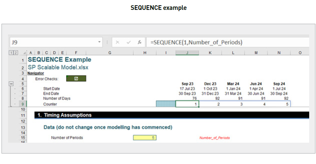
This formula will allow us to create a sequence of numbers from one [1] to the value of Number_of_Periods. We use two arguments to cite that the formula should spill over one row and Number_of_Periods columns. If we enter “10” into the Number_of_Periods cell, we will expand our counter from five [5] to ten [10], as shown in the screenshot “SEQUENCE Expansion Example”.
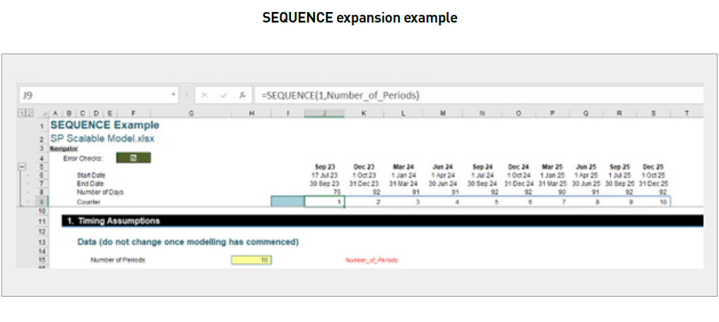
This can work with other calculations, not just date formulas. Overall, the use of dynamic arrays is a powerful tool when building a scalable financial model. By taking advantage of the flexibility and efficiency they provide (eg, range names calculating only once, being able to vary dimension lengths), we can create a model that can adapt to changes in the data and provide valuable insights for the business.
2. INDIRECT function
Another way to scale up the model is by using the INDIRECT function. The INDIRECT function refers to cells indirectly, which means the cell reference is determined by the contents of another cell or formula. Essentially, INDIRECT works as shown in the screenshot “INDIRECT Function Basic Concept”.
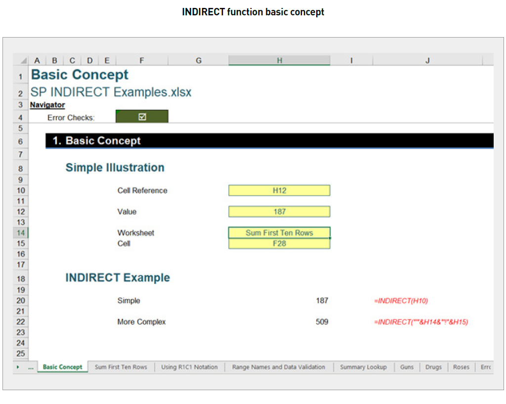
The formula in cell H12 (showing the value 187) is:
=INDIRECT(H10).
With only one argument in this function, INDIRECT assumes the A1-cell notation (eg, the cell in the tenth row, eighth column is cell H10). Note that the value in cell H10 is H12; this formula returns the value/contents of cell H12, ie, 187. This can be especially helpful when we have a large dataset or a complex model that requires frequent updates.
One way to use the INDIRECT function in a scalable model is to create dynamic references to other sheets or workbooks. For example, we may use the INDIRECT function to reference a sheet name that is stored in a cell, rather than hard-coding the sheet name into a formula. This makes it easier to update the model when we add or remove sheets without having to update the formulas manually.
For example, we have typed our sheet name into cell G10 (given the range name Selection) and we use the following formula to extract the Revenue for the first period of the Apples sheet (using a fruit theme) (see also the screenshot “INDIRECT Example”):
=INDIRECT(“‘”&Selection&”‘!RC”,FALSE)
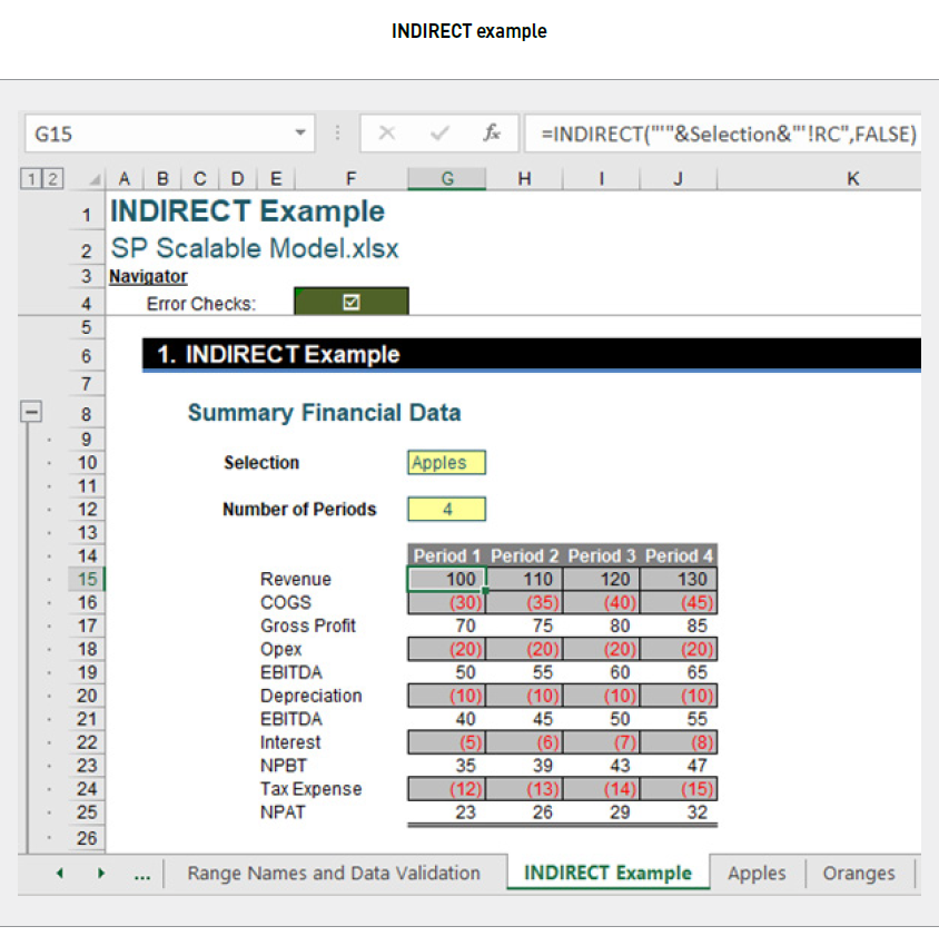
Here, we are using R1C1 cell reference approach, which means this part of the formula “‘”&Selection&”‘!RC” will refer to ‘Apples’!RC, which is the same current cell (G15) but for a different worksheet. The second argument of the INDIRECT function will determine the referencing methodology we use here. Hence, R1C1 will be used here as we set the second argument of INDIRECT to FALSE.
Another way to use the INDIRECT function in a scalable model is to reference ranges that change in size or location. We can use the INDIRECT function to reference a range of cells that is determined by the result of another formula. Using the same previous example, we can add an input called Num_Of_Periods. Then, we will modify our R1C1 reference within the formula to make it into a dynamic array, which gets all four [4] Revenue periods here:
=INDIRECT(“‘”&Selection&”‘!RC:RC[“&Num_Of_Periods-1&”]”,FALSE)
See the screenshot “INDIRECT Modified Example”.

The part “‘”&Selection&”‘!RC:RC[“&Num_Of_Periods-1&”]” will evaluate to ‘Apples’!RC:RC[3], which refers to the same current cell G15 and the three [3] cells next to it, which is the range G15:J15 in the Apples worksheet.
However, it is worth noting that the use of the INDIRECT function can also have drawbacks in terms of performance and stability. In large models with many INDIRECT functions, the calculation time may become significantly longer because Excel needs to evaluate all the indirect references. Additionally, if we change the structure of the workbook, such as renaming or moving sheets, the INDIRECT function may return errors, which can be difficult to debug. It is also a volatile function, which means it recalculates all the time and may be seen as an inefficient use of computing resources.
Overall, although the INDIRECT function may be a powerful tool for creating scalable models, it is important to use it cautiously and be aware of its potential limitations and drawbacks.
3. Tables
Tables (Insert -> Table or CTRL + T) represent a powerful feature in Excel that can help to manage data efficiently. They provide many benefits that can help to create a scalable and flexible financial model quickly.
One benefit of using Tables in a model is that it updates/extends/reduces everything automatically. A Table will usually update the format or formula(s) inside the Table when we are adding or removing data. For example, we have a simple Table called “Date” shown in the screenshot “Table Example”.
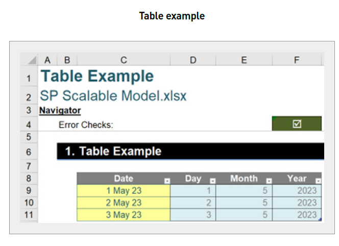
When we add “4 May 2023” to the cell below cell C11, the Table will update the format accordingly (see the screenshot “Updated Table”).
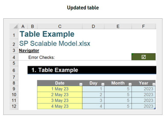
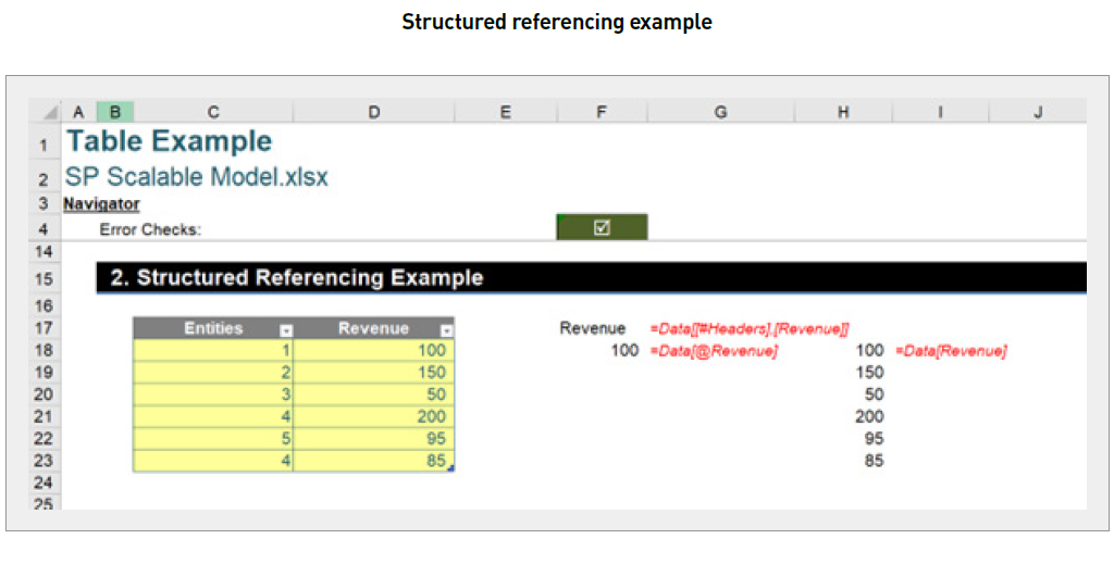
This feature helps in creating a scalable model if we want to add more inputs into the model with similar calculation logic. Besides automatically updating features of Tables, structured referencing (the syntax of Excel Tables) may also assist when creating an Excel scalable model. This feature allows the user to refer to cells in the Table using descriptive names (Table and column/field names) instead of cell references. This makes it easier to write and understand formulas, and it reduces the risk of errors. For instance, if we create an Excel Table named “Data” when we want to refer to all the data within the Revenue field, we simply type:
=Data[Revenue]
When we want to refer to the headings of the Table, we use the following formula:
=Data[[#Headers],[Revenue]]
When we want to refer to same row data of the Table, we use the @ symbol (see the screenshot “Structured Referencing Example”).
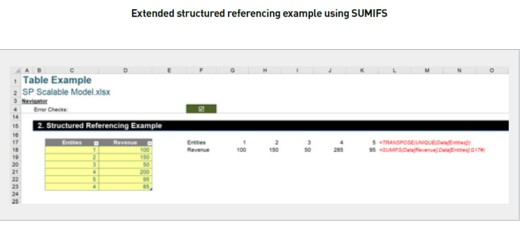
We can use Table data in conjunction with either the SUMIFS or SUMIF function to make our model scale dynamically (see the screenshot “Using Structured Referencing and SUMIFS”).
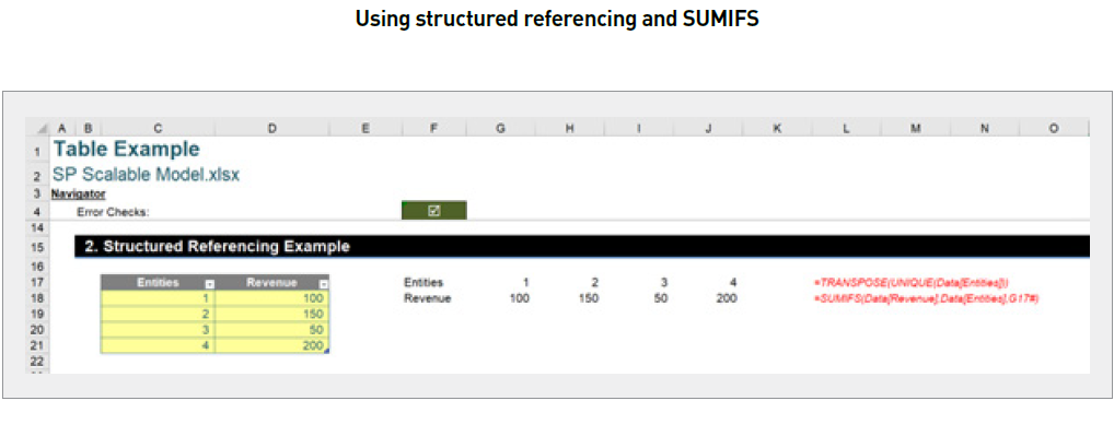
For example, we can use the following formulas to calculate the sum of revenue of each entity:
The following formula will generate the unique list of entities:
=TRANSPOSE(UNIQUE(Data[Entities]))
The following formula will sum up all the revenue of all entities:
=SUMIFS(Data[Revenue],Data[Entities],G17#)
If we add other entities or another revenue line for existing entities, the model will grab data directly related to these formulas. In
the example shown in the screenshot “Extended Structured Referencing Example Using SUMIFS”, we have added two [2] more lines.
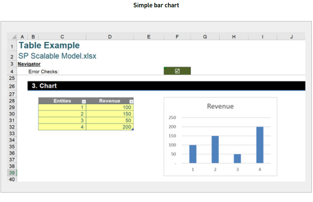
Another benefit of using Tables in an Excel scalable model is that they may be used to create dynamic charts. By selecting the Table and inserting a chart, we can create a dynamic chart that automatically updates as we add or remove data from the Table. This makes it easy to visualise changes in data over time and identify trends and patterns.
For example, we created a simple bar chart using the Chart_Data Table (see the screenshot “Simple Bar Chart”).
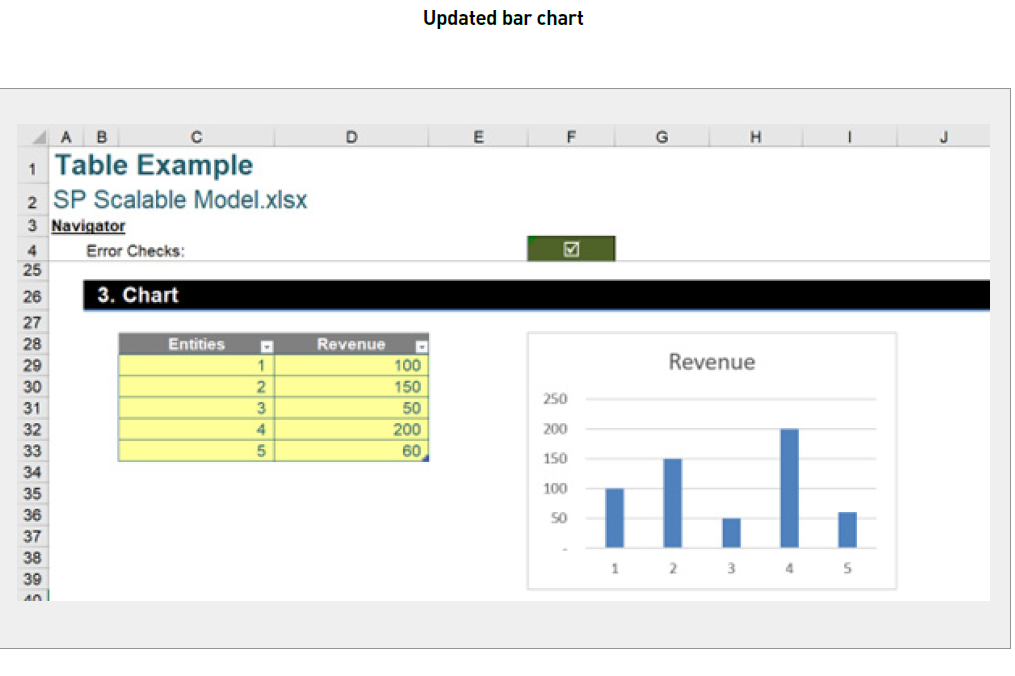
If we enter new entities in cell C33, we will see that our chart is updated as well (see the screenshot “Updated Bar Chart”).
4. Sum across multiple sheets
Excel provides several powerful features to simplify financial modelling. One of the most useful is the ability to sum across multiple sheets. This technique is especially useful when we need to create consolidated financial statements or when we anticipate adding more entities to our model in the future using a template sheet.
To illustrate, let’s say we have financial statements for multiple entities in our Excel workbook, with each entity represented by a separate sheet in our workbook (Entity 1, Entity 2, and Entity 3). In these sheets, we set up everything including the assumptions, calculations, and financial statements (outputs) so that every cell location is identical. Before we sum the values across all the entity sheets, we can create a Start sheet and an End sheet that surround the entity sheets and that we keep completely blank. The Start sheet should be the leftmost sheet to the entities, and the End sheet should be the rightmost sheet to the entities (see the screenshot “Multiple Sheets”).

If we wish to sum the values in cell F14 on each entity sheet to get the total operating expenditure (Opex) for all entities (see the screenshot “Consolidated Summary Financial Data”), we can use the following formula:
=SUM(Start:End!F14)
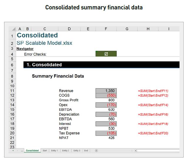
If we later need to add entities, we can simply put these new entity sheets between the Start and End sheets, and the formula will automatically update to include the new entities (we will need to ensure new entities have the same structure/cell locations as the previous sheets).
5. Reusing components
Sometimes, the modeller may look for parts of the model that can be reused in different sections of the same worksheet, other worksheets, or even different workbooks. These reusable components can include formulas, blocks of formulas, tables, Tables, or named ranges.
For example, we can duplicate the calculation of days receivable into a days payable computation because these calculations are quite similar. Another example may be where a user creates a template sheet and reuses that to help them build the model. There are certainly many ways we can reuse the model. Hence, it is important to model in a certain way to make it easier to reuse the components. One way to achieve that is to step out the calculation into smaller steps, avoiding combining everything into one massive formula, which might make the calculation hard to read or understand, thus reducing the reusability rate of such a formula.
6. Power Query and Power Pivot
A scalable model may become slow when more data is added to the model. Hence, Excel provides two powerful tools — Power Query (Get & Transform) and Power Pivot — to manage the increasing amounts of data.
Power Query allows users to extract, transform, and load one or more data sources into a workbook. If we set up the data transformation process in Power Query, we can automate this transformation process in the future whenever new data is added to the folder. This improves the performance of the scalable model when the data is extended.
Power Pivot is a powerful tool that allows users to deal with large datasets and perform complex calculations quickly. With the proper set-up, you can optimise scalable models that manage large datasets well. This may be achieved by referencing using dynamic arrays, not repeating key calculations, PivotTables, and ensuring datasets are not unnecessarily replicated.
Word to the wise
In summary, a combination of techniques is needed to truly build a scalable financial model in Excel. Dynamic formulas, Tables, reusing components/sections, and using Power Query and/or Power Pivot for large datasets all contribute to a maintainable model that may grow in multiple dimensions. We are conscious that there are more tools, techniques, and tricks other than those mentioned here — so happy exploring.
Liam Bastick, FCMA, CGMA, FCA, is director of SumProduct, a global consultancy specialising in Excel training. He is also an Excel MVP (as appointed by Microsoft) and author of Introduction to Financial Modelling and Continuing Financial Modelling. Send ideas for future Excel-related articles to him at liam.bastick@sumproduct.com. To comment on this article or to suggest an idea for another article, contact Oliver Rowe at Oliver.Rowe@aicpa-cima.com.


