New Excel function redefines formula building

Now, not just Mary can have a little LAMBDA.

For those in Office 365 Beta, Microsoft recently made a fantastic announcement for Excel. Only two weeks after LET was made Generally Available, its sister function, LAMBDA, was released into the wild. The power of this latest addition to the Excel family of functions cannot be overstated. This is going to revolutionise how you build formulas in Excel.

This function “completes” Excel (more on that below), as a key programming feature — missing forever in the world’s favourite spreadsheet software — is now made available, as well as the ability to create your own reusable formulas.

Confusingly, LAMBDA has nothing whatsoever to do with previous Greek-named functions such as BETA and GAMMA. The name dates back to Alonzo Church, a mathematician and logician who made major contributions to mathematical logic and the foundations of theoretical computer science. He coined the term as part of lambda calculus, in which all functions were deemed “anonymous”, ie, one that is not bound to an identifier. If this means nothing to you and you are now possessing a glazed expression, don’t worry, welcome to my world.

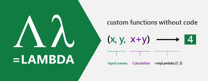
Simply put, LAMBDA allows you to define your own custom functions using Excel’s formula language. It’s user-defined functions without a Ph.D. in VBA or JavaScript. In Office 365 Beta, LAMBDA allows you to define a custom function in Excel’s very own formula language. Moreover, one function can call another (including itself), so there is no limit to the power you can deploy with a single function call. And as Microsoft states: “For folks with a computer science background, you’re probably already familiar with the concept of lambdas, and the introduction of LAMBDA makes the Excel formula language Turing Complete.” You can now sleep at night.

With LAMBDA, you can take any formula you’ve built in Excel and wrap it up in a LAMBDA function and give it a name (like “CUSTOM1”). Then, anywhere in your Excel workbook, you can refer to CUSTOM1, reusing that custom function throughout your sheet.

So here’s the rub. If you create such a LAMBDA called CUSTOM1, you can call CUSTOM1 within the definition of CUSTOM1. This is known as “recursion”, and this is what “completes” Excel. This is something that before was only possible in Excel through script (like VBA/JavaScript). This is what makes LAMBDA functions so powerful (again, see below).

Reusable custom functions

One of the more challenging parts of working with formulas in Excel is that you often get fairly complex formulas that are reused numerous times through the sheet (often by just copying/pasting). This can make it hard for others to read and understand what’s going on, put you more at risk of errors, and make it hard to find and fix the errors. With LAMBDA, you have reuse and composability. Create libraries for any pieces of logic you plan to use multiple times. It offers convenience and reduces the risk of errors.

So how does it work?

The syntax of LAMBDA is perhaps not the most informative: LAMBDA(parameter_or_calculation, …)

That’s, er, great. Perhaps a run-through might be best.

There are three key pieces of =LAMBDA to understand:

1. LAMBDA function components.
2. Naming a LAMBDA.
3. Calling a LAMBDA function.

1. LAMBDA function components

Let’s take a simple example. Consider the following formula: =LAMBDA(x, x+1).

This is a very exciting formula in which we have x as the argument (oh no it isn’t, oh yes it is — see, I told you it was an argument), which you may pass in when calling the LAMBDA, and x+1 is the logic/operation to be performed.

For example, if you were to call the LAMBDA function above and define x as equal to five (5), then Excel would calculate 5 + 1 = 6, right?

Nope. You would get #CALC! Oops. That’s because it’s not quite as simple as that. You need to name your little LAMBDA.

2. Naming a LAMBDA

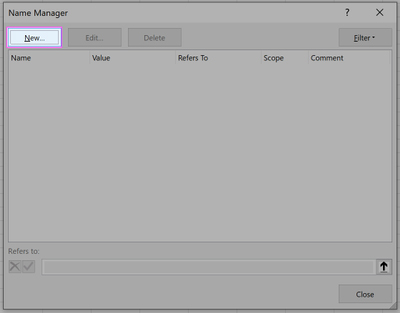
To give your LAMBDA a name so it can be reused, you have to use the Name Manager (Ctrl+F3 or go to Formulas > Name Manager on the Ribbon):

Once you open the Name Manager, the following dialog box will open:

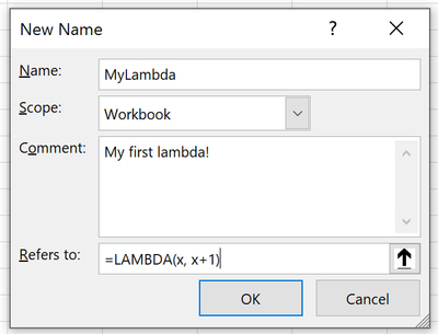
Click on New and fill out the related fields, as shown in the screenshot below.

To be clear:

• Name: The name of your function (this is where you name it).
• Comment: A description and associated ToolTip, which will be shown when calling your function.
• Refers to: Your LAMBDA function definition (this is where you put your formula — not in the Excel worksheet!).

Once you are finished, press OK to store your LAMBDA, and you should see the definition returned in the resultant window.

3. Calling LAMBDA

Now that you have done this, your first new LAMBDA function may be called in just the same way as every other Excel function is cited. For example, =MYLAMBDA(5) would equal six (6) and not #CALC! as before.

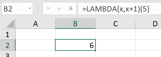
You don’t have to do it this way, though, if you don’t want to. You may call a LAMBDA without naming it. If we hadn’t named this marvellous calculation and simply authored it in the grid as we had first attempted, we could call it by simply typing =LAMBDA(x, x+1)(5), as shown in the screenshot below.

The sky’s the limit. You are not restricted to just numbers and text. You can also use:

• Dynamic arrays: Rather than passing a single value into a function, you can pass an array of values, and functions can also return arrays of values.
• Data types: The value stored in a cell is no longer just a string or a number. A single cell can contain a rich data type with a large set of properties.

Functions can take data types and arrays as arguments, and they can also return results as data types and arrays. The same is true with the LAMBDAs you build.

To show you just how useful these functions are, I want to finish with recursion. To show you just how useful these functions are, I want to finish with recursion. To show you … well, you get the idea.

Recursion: Making the right call

One of the big missing pieces in Excel formulas has been the ability to loop or create a function that calls itself. This is something modellers have wanted for years with common calculations such as calculating optimum debt while taking account of interest and other similar iterative computations. Where you can, it is often better to solve formulaically (eg, calculating interest using simultaneous equations), but sometimes you find yourself in a situation screaming for a LAMBDA function.

Here is an example that Microsoft came up with to demonstrate the idea.

Imagine you have a set of text strings and want to specify which characters should be removed from those strings dynamically:

Because the set of characters you’re specifying are not static, there really isn’t any good way of doing this. The goal for the Desired Result column is blank cells, not what it shown above. If you knew it was always a fixed set of characters, you could calculate using nested logic, but that would be pretty complex and error prone to author.

With LAMBDA, you could create a function called REPLACECHARS that references itself allowing you to iterate over the list of characters to be removed, where REPACECHARS has been defined as

=LAMBDA(textString, illegalChars, IF(illegalChars="", textstring, REPLACECHARS(SUBSTITUTE(textString, LEFT(illegalChars, 1), ""),RIGHT(illegalChars, LEN(illegalChars)-1))))

Notice that in the definition of REPLACECHARS, there is a reference to REPLACECHARS! The IF statement says if there are no more illegal characters, return the input textString and otherwise remove each occurrence of the leftmost character in illegalChars. Recursion kicks in with the request to call REPLACECHARS again with the updated string, and the rest of illegalChars. This means it will keep calling itself until it has parsed over every character to be removed, giving the desired result.

Points to note

- LAMBDA doesn’t have to be used in a named range, as shown above. You must remember to pass the required parameters to avoid the #CALC! error, eg,

=LAMBDA(x, x+1)(5)

will return six (6) if entered in a cell.

- LET requires at least one variable to work; LAMBDA can take between zero (0) and 253 variables (eg, an exception to the first point is =LAMBDA(RAND()), which will work).

- LAMBDA inside a LET function will work, eg,

=LET(CUSTOM1, LAMBDA(x, x+1), CUSTOM1(5))

will return six (6) if entered into a cell:

- When you begin writing a LAMBDA function, the Intellisense is presently working inside all LAMBDA parameters except for the first one (Microsoft would like to know if that’s not the behaviour any reader sees). Of course, Intellisense should also work for the first parameter, but there is presently a bug, which will be fixed shortly.

Word to the wise

The best thing is just to get going with this powerful addition to the Excel vocabulary. The LAMBDA function is available to members of the Insiders Beta program running Windows and Mac builds of Excel 365. It might just be a time to upgrade if you don’t already have it.

— Liam Bastick, FCMA, CGMA, FCA, is director of SumProduct, a global consultancy specialising in Excel training. He is also an Excel MVP (as appointed by Microsoft) and author of Introduction to Financial Modelling. Send ideas for future Excel-related articles to him at liam.bastick@sumproduct.com. To comment on this article or to suggest an idea for another article, contact Jeff Drew, an FM magazine senior editor, at Jeff.Drew@aicpa-cima.com.