Excel unveils function that improves on VLOOKUP

Editor’s note: Microsoft announced 29 October 2019 that it has changed the order of arguments for XLOOKUP. For more details, visit techcommunity.microsoft.com.

Ask any accountant and they will tell you two “truths”:

1. They are a better-than-average driver, and everyone else is an idiot on the roads.
2. They are a better-than-average Excel user because they know how to use VLOOKUP.

It should be noted here that I hate VLOOKUP with a passion, and if anything can hurry its demise, well, I shall welcome it with open arms. Ladies and gentlemen, may I present the future of looking up for the masses — XLOOKUP? Hopefully, it will make an “ex” of VLOOKUP!

Before we continue, let me clarify that Microsoft has added two new functions, XLOOKUP and XMATCH. For reasons that will become clear, here we will mainly consider the former function — because once you understand XLOOKUP, XMATCH becomes obvious (nothing personal, XMATCH).

Meet the new boss, not the same as the old boss

XLOOKUP has been released in what Microsoft refers to as “Preview” mode; ie, it’s not yet “Generally Available”, but it is something you can hunt out. Presently, just like Dynamic Arrays, you need to be part of what is called the “Office Insider” programme, which is an Office 365 fast track. You can register in File > Account > Office Insider in Excel’s backstage area, as shown in the screenshot below.

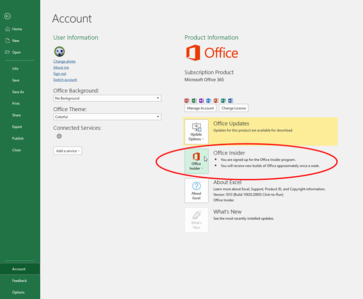
Even then, you’re not guaranteed a ticket to the ball, as only some will receive the new function as Microsoft slowly rolls out these features and functions. Please don’t let that put you off. This feature will be with all Office 365 subscribers soon.

XLOOKUP basics

XLOOKUP has the following syntax:

XLOOKUP(lookup_value, lookup_vector, results_array, [match_mode], [search_mode])

On first glance, it looks as if it has too many arguments, but often you will only use the first three:

• lookup_value: This is required and defines what value you want to look up.
• lookup_vector: This reference is required and is the row or column of data you are searching to look up lookup_value.
• results_array: This is where the corresponding item is you wish to return and is also required (even if it is the same as lookup_vector). This does not have to be a vector (ie, one row or one column of cells); it may be an array (with at least two rows and at least two columns of cells). The only stipulation is that the number of rows/columns must equal the number of rows/columns in the column/row vector. In other words, if lookup_vector is a row vector, then the number of columns must be equal; if lookup_vector is a column, then the number of rows in both must be identical.
• match_mode: This argument is optional and offers four choices:
  • 0: Exact match (default);
  • -1: Exact match or else the largest value less than or equal to lookup_value;
  • 1: Exact match or else the smallest value greater than or equal to lookup_value; and
  • 2: Wildcard match. You should use the special character ? to match any character and * to match any run of characters.

What’s impressive, though, is that for certain selections of the final argument (search_mode), you don’t need to put your data in alphanumerical order! As far as I know, this is a first for Excel.

• search_mode: This argument is also optional. There are again four choices:
  • 1: Search first to last (default);
  • -1: Search last to first;
  • 2: What is known as a binary search, first to last (requires lookup_vector to be sorted). Just so you know, a binary search is a search algorithm that finds the position of a target value within a sorted array. A binary search compares the target value to the middle element of the array. If they are not equal, the half in which the target cannot lie is eliminated and the search continues on the remaining half, again taking the middle element to compare to the target value and repeating this until the target value is found; and
  • -2: Another binary search, this time last to first (and again, this requires lookup_vector to be sorted).

XLOOKUP compares favourably with VLOOKUP

While VLOOKUP is the third-most-used function in Excel (behind SUM and AVERAGE), it has several well-known limitations that XLOOKUP overcomes. Specifically, VLOOKUP:

• Defaults to an “approximate” match: Most often, users want an exact match, but this is not VLOOKUP’s default behaviour. To perform an exact match, you need to set the final argument to FALSE. If you forget (which is easy to do), you’ll probably get the wrong answer;
• Does not support column insertions/deletions: VLOOKUP’s third argument is the column number you’d like returned. Since this is a hard-coded number, if you insert or delete a column, you need to increment or decrement the column number inside the VLOOKUP — hence the need for the COLUMNS function (and the corresponding ROWS function for HLOOKUP);
• Cannot look to the left: VLOOKUP always searches the first column, then returns a column to the right. There is no way to return values from a column to the left, forcing users to rearrange their data;
• Cannot search from the bottom: If you want to find the last occurrence, you need to reverse the order of your data;
• Cannot search for next largest item: When performing an “approximate” match, only the item less than or equal to the searched item can be returned and only if correctly sorted; and
• References more cells than necessary: VLOOKUP’s second argument, table_array, needs to stretch from the lookup column to the results column. As a result, it typically references more cells than it truly depends on. This could result in unnecessary calculations, reducing the performance of your spreadsheets.

Let’s have a look at XLOOKUP versus VLOOKUP:

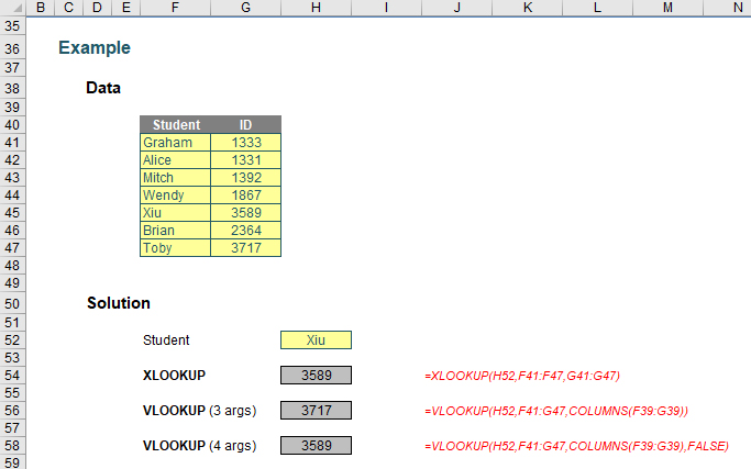
You can clearly see in the screenshot above that the XLOOKUP function is shorter:

=XLOOKUP(H52,F41:F47,G41:G47)

Only the first three arguments are needed, whereas VLOOKUP requires both a fourth argument, and, for full flexibility, the COLUMNS function as well. XLOOKUP will automatically update if rows/columns are inserted or deleted. It’s just simpler.

HLOOKUP has similar issues, as shown in the screenshot below.

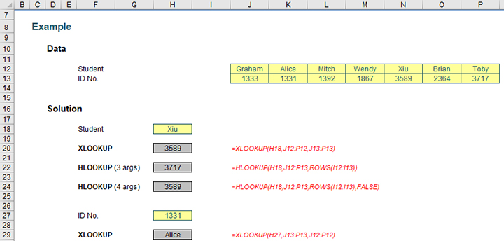
The above example highlights what happens if I try to deduce the student name from the Student ID. HLOOKUP cannot refer to earlier rows, just as VLOOKUP cannot consider columns to the left. Given that any unused elements of the table also are ignored, it’s just good news all around.

XLOOKUP changes all that. Indeed, things get even more interesting when you start considering XLOOKUP’s final two arguments, namely match_mode and search_mode, as shown in the screenshot below.

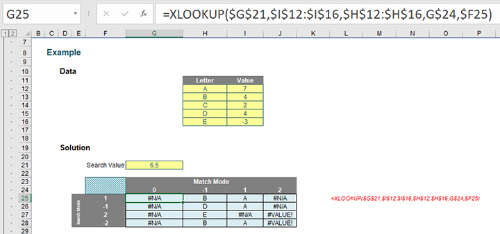
Notice that I am searching the “Value” column, which is neither sorted nor contains unique items. However, I can look for approximate matches — impossible with VLOOKUP and/or HLOOKUP.

Do you see how the results vary depending upon match_mode and search_mode?

The match_mode zero (0) returns #N/A because there is no exact match.

When match_mode is -1, XLOOKUP seeks an exact match or else the largest value less than or equal to the lookup_value (6.5). That would be 4 — but this occurs more than once (B and D both have a value of 4). XLOOKUP chooses depending upon whether it is searching top down (search_mode 1, where B will be identified first) or bottom up (search_mode -1, where D will be identified first). Note that with binary searches (with a search_mode of 2 or -2), the data needs to be sorted. It isn’t — hence, we have rubbish answers that cannot be relied upon.

With match_mode 1, the result is more clear-cut. Only one value is the smallest value greater than or equal to 6.5. That is 7, and is related to A. Again, binary search results should be ignored.

The match_mode 2 results are spurious. This is seeking wildcard matches, but there are no matches, hence #N/A for the only search_modes that may be seen as credible (1 and -1).

Clearly binary searches are higher maintenance. In the past, it was worth investing in them as they did return results more quickly. However, Microsoft says this is no longer the case: Apparently, there is “no significant benefit to using the binary search options”. If this is indeed the case, then I would strongly recommend not using them going forward with XLOOKUP.

To show how simple it now is to search from the end, consider the screenshot below:

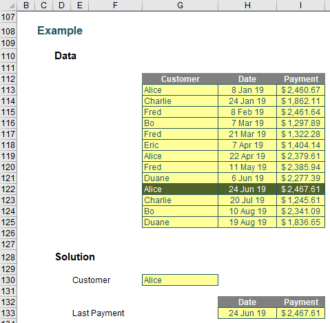
This used to be an awkward calculation — but not anymore! The formula is easy. To pull the date into cell H133, you use:

=XLOOKUP($G$130,$G$113:$G$125,H$113:H$125,,-1)

To pull the payment into cell I133, you simply copy the formula across one cell. This will replace the H’s with I’s:

=XLOOKUP($G$130,$G$113:$G$125,I$113:I$125,,-1)

This is a “standard” XLOOKUP formula, with a “bottom up” search coerced by using the final value of -1 (forcing the search_mode to go into “reverse”).

XLOOKUP has tons of potential uses — too many to cover in this article, but rest assured we will take another look at XLOOKUP soon. But before you go, let’s take a quick look at the other function that debuted with XLOOKUP.

A quick glance at XMATCH

XMATCH has arrived with a similar signature to XLOOKUP, but instead it returns the index (position) of the matching item. XMATCH is both easier to use and more capable than its predecessor, MATCH.

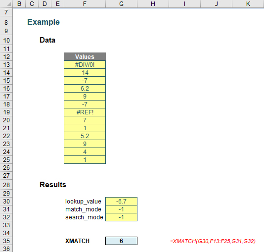
XMATCH has the following syntax:

XMATCH(lookup_value, lookup_vector, [match_mode], [search_mode])

Where:

• lookup_value: This is required and defines what value you want to look up.
• lookup_vector: This reference is required and is the row or column of data you are referencing to look up lookup_value.
• match_mode: This argument is optional. There are four choices:
  • 0: Exact match (default);
  • -1: Exact match or else the largest value less than or equal to lookup_value;
  • 1: Exact match or else smallest value greater than or equal to lookup_value; and
  • 2: Wildcard match. You should use the special character ? to match any character and * to match any run of characters.

Again, for certain selections of the final argument (search_mode), you don’t need to put your data in alphanumerical order.

• search_mode: This argument is also optional. There are again four choices:
  • 1: Search first to last (default);
  • -1: Search last to first;
  • 2: This is a binary search, first to last (requires lookup_vector to be sorted); and
  • -2: Another binary search, this time last to first (and again, this requires lookup_vector to be sorted).

As you can see, it’s a fairly straightforward addition to the MATCH family. It acts similarly to MATCH — just with heaps more functionality.

Word to the wise

XLOOKUP and XMATCH open up new avenues for Excel to explore, but it must be remembered they are still in Preview and may only be accessed by a lucky few on the Insider track. Feel free to download and play with this Excel file, but don’t be too perturbed if your version of Excel does not recognise these functions yet.

— Liam Bastick, FCMA, CGMA, FCA, is director of SumProduct, a global consultancy specialising in Excel training. He is also an Excel MVP (as appointed by Microsoft) and author of Introduction to Financial Modelling. Send ideas for future Excel-related articles to him at liam.bastick@sumproduct.com. To comment on this article or to suggest an idea for another article, contact Jeff Drew, an FM magazine senior editor, at Jeff.Drew@aicpa-cima.com.