MOD-elling periodic transactions in Excel

If you build forecast models in which certain transactions occur periodically but not every period, then the MOD function might be for you.

For example, you might model monthly and pay tax quarterly; you may model quarterly yet pay dividends half-yearly, etc. This is where the MOD function comes in — even if it causes division among the financial modelling community.

The MOD function, MOD(Number,Divisor), returns the remainder after the Number (first argument) is divided by the Divisor (second argument). The result will have the same sign as the Divisor.

For example, 9 ÷ 4 = 2.25, or 2 remainder 1. MOD(9,4) is an alternative way of expressing this, and hence equals one (1) also. Note that the 1 may be obtained from the first calculation by (2.25 – 2) × 4 = 1, ie, in general:

MOD(n,d) = n - d*INT(n/d),

where INT() is the integer function in Excel.

This function has various uses, as evidenced by three common examples listed below.

1. Obtaining “residuals”: In some instances in modelling, you need the integer part of a number, eg, how many payments fall between two dates may calculate as 9.94 — but that’s nonsense. In this instance, you would have made only nine payments, ie, INT(9.94). Similarly, you might want to accrue the fee for payments not yet made. Using MOD(9.94,1) you would obtain the result 0.94, ie, the number after the decimal place. Note that 9.94 – INT(9.94) gives the same result here; the MOD approach is simply shorter.

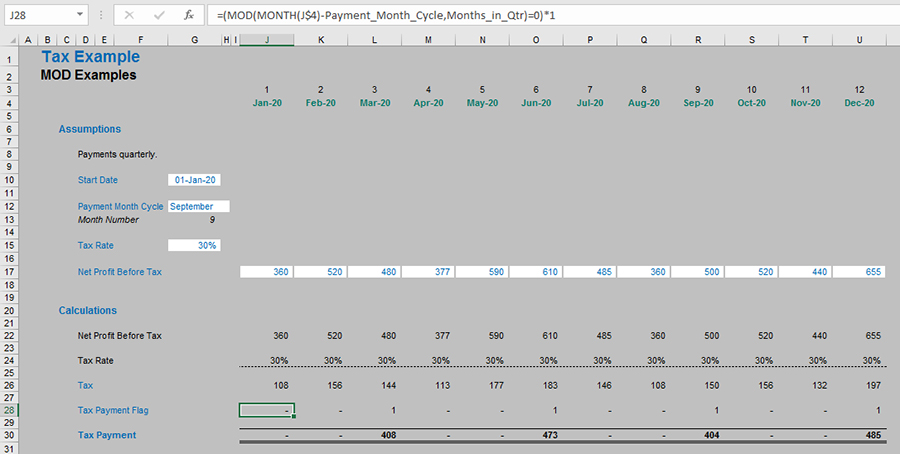
2. Calculations at regular time intervals: Consider the aforementioned tax payments as an example. Many companies make tax payments quarterly. If we assume these payments are made in March, June, September, and December, then we can formulate the payment as IF(MOD(Month_Number, Divisor)=0,Make_Payment,0), etc.

3. Summing every nth row: It is not uncommon for users to want to sum every nth cell (eg, second, third, fourth, …) in a spreadsheet. Excel has no standard function that will do this, but MOD can come to the rescue. For example, the array formula (obtained by pressing Ctrl+Shift+Enter to get the braces { and }),

{=SUM(IF(MOD($E$19:$E$48,$G$13)=0,$F$19:$F$48,0))}

was used in cell H53 in the following example:

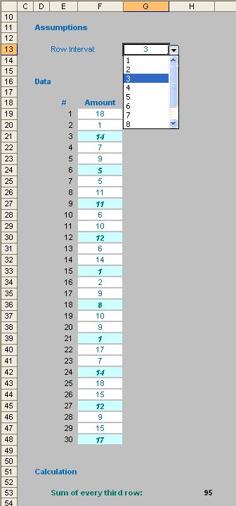
Arrays using large ranges can cause calculations to slow down considerably. This is why I used a counter rather than the volatile ROW() function (you may recall volatile functions calculate each time you press ENTER or F9).

An accuracy warning

If accuracy is vital, be careful with MOD, as it may give very slightly erroneous results, as shown in the following example, which you can find in this Excel file:

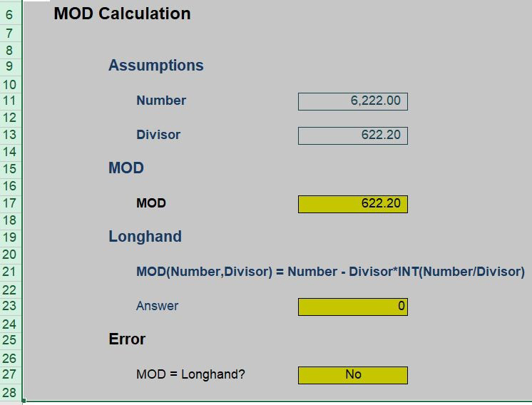
The result for MOD in cell G17 might seem inconsequential, but imagine you were making calculations based on MOD(Number,Divisor)=0. In this case MOD would not equal zero, and the calculation would not work.

This issue tends to occur more commonly when working with nonintegers.

The problem here isn’t really MOD. Calculations are performed in what is known as a binary [1,0] format, and many decimal numbers have no exact binary representation (just as 1/3 has no exact decimal representation). As an illustration, 10 times the binary approximation to 622.2 is

6222.0000000000004547....

ie, you may need to use the ROUND(Number,Num_digits) as part of your formula, too, in order to round your Number to Num_digits (number of digits after the decimal point).

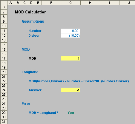
Note that the longhand approach also gives a result of -1.

Microsoft explains that this approach has been taken deliberately to be consistent with the competitor dBase software’s MOD function. If you always need MOD to deliver a value of x where 0 ≤ x < divisor, then use the adjusted formula:

=IF(MOD(Number,Divisor)<0,ABS(Divisor)+MOD(Number,Divisor)).

A practical use for MOD

Now that I have explained MOD, I can show you a really good use of this function for a situation that causes many working in finance plenty of consternation. You can download my Excel file with this solution, which works in conjunction with OFFSET. Let me just remind you of our old friend the OFFSET, as follows:

OFFSET(Reference,Rows,Columns,[Height],[Width]).

The arguments in square brackets (Height and Width) can be omitted from the formula in this instance. In its most basic form, OFFSET(Reference,x,y) will select a Reference x rows down (-x would be x rows up) and y rows to the right (-y would be y rows to the left).

Imagine you have set up a scenario table in Excel to determine which inputs should be used in your model (ie, “what-if? Analysis”):

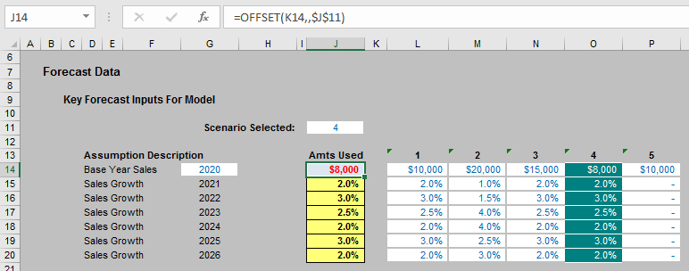
This method allows for various scenarios to be modelled easily with a different set of input data inserted into each column (from column L onwards in this illustration). A selector (cell J11 in the figure above) is used to select the active scenario, which may be highlighted using conditional formatting (see later).

The data used to drive the model is then highlighted in column J (here, emphasised in yellow) using the following formula, for cell J14 in this example:

=OFFSET(K14,,$J$11)

In other words, this formula looks up data x columns to the right of column K, where x is specified as the value input in cell J11 (here, this value is 4 so column O’s data is selected).

Clearly, using a columnar approach here makes it very straightforward to set the various scenarios out. However, most financial models are displayed with dates going from left to right across columns rather than down the page using rows. This requires us to transpose the data, and again we may use OFFSET to transpose the data:

Here, the period numbers specified in row 31 make it easy for us to transpose the data. For example, the formula in cell L34 would be:

=OFFSET($J$13,L$31,)

ie, insert the data x rows down from cell J13 in the first graphic, where x is again specified as the value input in cell J11.

Take care, however, if using an amount-followed-by-growth-rates approach for forecast/budget data. The amounts using these examples should be as follows:

The correct formula here is:

=IF(L$31=1,L$34,K36*(1+L$34))

for cell L36 (for example), ie, if it is the first period, take the amount; otherwise take the amount calculated in the preceding period and multiply it by (1 + growth rate specified in the current period, not the next period).

When actual data is inputted into a model, it frequently replaces the original information. Management, therefore, loses the ability to see how accurate forecasts were originally and how budgeting may be improved. One way around this would be to simply have “Actuals” as one of the scenarios so that all forecasts are retained. This is often all that is required, and if so, simply do that.

However, often we may wish to undertake variance analysis by comparing actual data with the original budgeted information. In this case, I would suggest the following approach.

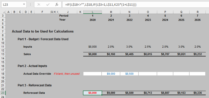
Rows 9 to 13 in the screenshot above simply reiterate the calculations already detailed earlier regarding the original forecasting. Note row 18, however: This is where actual data is added instead. In this example, I simply use hard-coded inputs for my data, but it only requires a simple variation to this methodology to revise growth rates, etc.

Using my logic, we simply use actual data where it is available; otherwise, we fall back on the original data and calculations. This is achieved by the formula in row 23 in my example, which is (for cell L23):

=IF(L$18<>"",L$18,IF(L$3=1,L$11,K23*(1+L$11))),

ie, if there is data in the corresponding cell in row 18, use it; if not, if it is the first period take the original input value, otherwise simply inflate the prior-period amount by (1 + growth rate for that period). It may include a nested IF statement, but it is still a relatively simple and straightforward calculation.

Performing the calculations is only half the battle. Modellers often have difficulty comparing the original outputs with the reforecast counterparts in an effective and efficient manner. If sufficient, the following would be relatively straightforward:

This is very easy to put together, but alas, more often than not, senior management requires the following presentation instead:

Seem familiar? I have been a model reviewer for many a year and have seen this type of output on an extremely regular basis. Many senior management teams like it this way, and it is not my role to challenge the status quo — it doesn’t stop me from trying, though!

The problem with this layout is that it lends itself to promoting poor practice. Modellers tend to a large number of unique formulas across a row, which in turn slows down model construction and increases the potential for mistakes, such as referencing errors.

If you have to use this layout, try creating the simple summary elsewhere (maybe on an input page).

Look carefully at this graphic. The shading in cell K28 above may appear innocuous, but it is the most important cell on the worksheet and has been named BC_Sales_Summary accordingly (BC means “Base Cell” for an OFFSET function). Consider:

• For every column moved to the right, the cursor is in a different year. One column across is year 1, two columns across is year 2, and so on
• For every row moved down, the cursor reports a different figure. One row down is the Budget data, two rows down is the Actual/Reforecast data, and three rows down is the Variance. The depth of this table (three rows) has been defined as List_Depth so that it may be used in formulas.

Now, if we return to the outputs worksheet and modify it slightly by inserting two additional lines and using the OFFSET function, your potential troubles may become a thing of the past, as shown below.

You will see that each row of the revised output example contains only one unique formula copied across, making it easy to edit, extend, and review. This is achieved by adding two rows:

• Selector (row 7): Identifies whether the column should be reporting the budget information, the actual data, or the variance. The equation used makes use of the MOD function:
  
  =MOD(L$4-1,List_Depth)+1
  
  As stated above, List_Depth is the number of selections (Budget, Act / Ref’cast, Variance) permissible — in this case three. The formula =MOD(L$4,List_Depth) takes the counter and converts each one to 1, 2, and zero (ie, the remainder upon dividing the counter by three). By subtracting one inside the MOD function and adding it once more outside, this simply forces a zero to a three instead, so that the Selector reports the values 1, 2, and 3 alternately.

• Year No. (row 8): Simply notes which year the column is reporting using the formula:
  
  =IF(L$7=1,K8+1,K8),
  
  ie, the year increases the period that the counter in row 7 equals 1 (in this example).

Therefore, in my example, row 13 requires a very simple formula to generate the required outputs:

=OFFSET(BC_Sales_Summary,L$7,L$8).

For example, cell Q13 equals OFFSET(BC_Sales_Summary,3,2), which would refer to the year 2 Variance figure of $840.

Easy! See for yourself: You can check all of our examples in these two workbooks: SP MOD Examples and SP Actual vs. Budget Examples.

— Liam Bastick, FCMA, CGMA, FCA, is director of SumProduct, a global consultancy specialising in Excel training. He is also an Excel MVP (as appointed by Microsoft) and author of Introduction to Financial Modelling. Send ideas for future Excel-related articles to him at liam.bastick@sumproduct.com. To comment on this article or to suggest an idea for another article, contact Jeff Drew, an FM magazine senior editor, at Jeff.Drew@aicpa-cima.com.