CHOOSE carefully with this Excel function

Accountants building financial models can select from several functions to track down data in a spreadsheet. In recent months we devoted three columns to examining the following choices: VLOOKUP and HLOOKUP, the combination of INDEX and MATCH, and LOOKUP. This month’s article looks at another similar function, one you can CHOOSE but often may not want to.

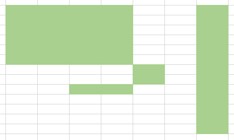
CHOOSE is a function used in modelling but, perhaps, not as regularly as some others. CHOOSE is useful for noncontiguous references, as illustrated in the screenshot below.

Just so that we are clear on jargon: A noncontiguous range (with reference to Excel) means a range that cannot be highlighted with the mouse alone. In the image above, to highlight the cells coloured, you would have to press the Ctrl key as well.

INDEX, LOOKUP, VLOOKUP, and HLOOKUP all require contiguous references. They refer to lists, row vectors, column vectors, and/or arrays. CHOOSE is different: =CHOOSE(index_number, value1, [value2]…).

CHOOSE allows references to different calculations, workbook/worksheet references, etc. This versatility can make CHOOSE an enticing option, but I would advise using discretion when determining if CHOOSE is the best function to use. To understand why, you need to have a grasp on how CHOOSE works.

CHOOSE uses index_number to return a value from the list of value arguments. Modellers can use CHOOSE to select one of up to 254 values based on the index number (index_number). For example, if value1 through value7 are replaced with the days of the week:

=CHOOSE(index_number, “Sunday”, “Monday”, “Tuesday”, “Wednesday”, Thursday”, “Friday”, “Saturday”)

this formula returns one of the days when a number between 1 and 7 is used as index_number.

The CHOOSE function employs the following syntax to operate:

CHOOSE(index_number, value1, [value2])

The function has the following arguments:

• index_number: This is required and used to specify which value argument is to be selected. The argument index_number must be a number between 1 and 254, or a formula or reference to a cell containing a number between 1 and 254:
  • If index_number is 1, CHOOSE returns value1; if it is 2, CHOOSE returns value2; and so on.
  • If index_number is less than 1 or greater than the number of the last value in the list, CHOOSE returns the #VALUE! error value.
  • If index_number is a fraction, it is truncated to the lowest integer before being used.
• value1, value2, ...: value 1 is required, but subsequent values are optional. There may be between 1 and 254 value arguments from which CHOOSE selects a value or an action to perform based on index_number. The arguments can be numbers, cell references, defined names, formulas, functions, or text.

It should be further noted that:

• If index_number is an array, every value is evaluated when CHOOSE is evaluated.
• The value arguments to CHOOSE can be range references as well as single values.

It is important to consider carefully when it is appropriate to use CHOOSE. I am pickier about using CHOOSE than many. For instance, a well-known Excel website proposes the following formula for calculating the US Thanksgiving date:

=DATE(A1,11,CHOOSE(WEEKDAY(DATE(A1,11,1)),26,25,24,23,22,28,27))

To understand this formula, assume that cell A1 contains the year and note that DATE(Year,Month,Day) returns a date and WEEKDAY(Date) returns a number 1 (Sunday) through 7 (Saturday). The formula works, but doesn’t it look horrible? It is full of hard code and contains an unnecessary number of arguments. The formula could exclude CHOOSE and be rendered as: =DATE(A1,11,28-MOD(WEEKDAY(DATE(A1,11,1))+1,7)).

Now let me be clear here. I am not saying this is a simple, transparent formula, but test it against the CHOOSE option. Both formulas provide the same answer. CHOOSE — and plenty of additional hard code — has been used unnecessarily.

That’s not to say there isn’t a time and a place for CHOOSE. It is useful when you need to refer to cells on different worksheets or in other workbooks. But it’s more often not the best choice.

For example, some argue that CHOOSE is useful when a calculation needs to be computed using different methods, eg, =CHOOSE(index_number, calculation1, calculation2, calculation3, calculation4).

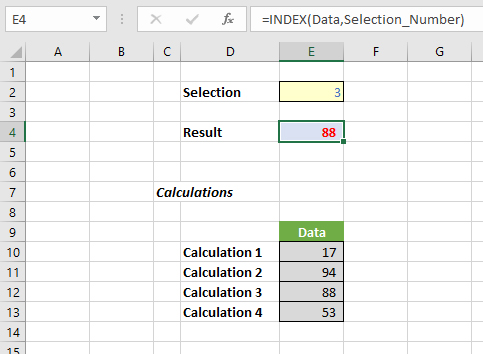
I disagree, and here’s why. In the example below, I have created a lookup table in cells E10:E13 that I have called Data (to create a range name, simply select the cell(s) and type the name into the “name box”, which is the area to the left of the formula bar). The calculations are all visible on the worksheet, rather than hidden away in the formula bar. The index_number selection, here referred to as Selection_Number, is inputted in cell E2. The formula, which is clearly visible in cell E4, is =INDEX(Data,Selection_Number). The INDEX formula produces the same result as the CHOOSE formula in the previous paragraph, but it is much more transparent and easier to follow.

I have taught financial modelling to many gifted analysts over the years, and a common mistake they make is building models that are easy to build rather than models that are easy to understand. The end user is the customer. The spreadsheet should be simple for the end user to use: Taking shortcuts in building the model invariably helps only the modeller — and even then, more often than not, shortcuts will backfire.

CHOOSE can lead to opaque models that need to be rebuilt and are often less flexible to use. So CHOOSE wisely.

— Liam Bastick, FCMA, CGMA, FCA, is director of SumProduct, a global consultancy specialising in Excel training. He is also an Excel MVP (as appointed by Microsoft) and author of An Introduction to Financial Modelling. Send ideas for future Excel-related articles to him at liam.bastick@sumproduct.com. To comment on this article or to suggest an idea for another article, contact Jeff Drew, an FM magazine senior editor, at Jeff.Drew@aicpa-cima.com.