Excel: 2 new errors and a SINGLE function

Editor’s note: Microsoft recently announced a rewrite of part of Excel’s calculation engine. The result is an evolutionary leap that promises to bring numerous improvements to Excel users in the coming years. Already unveiled are a new type of calculation (Dynamic Arrays), seven new functions, and two new errors. These changes have not yet been rolled out to all Excel users, but you don’t have to wait to see what they can do. Excel MVP Liam Bastick is covering all the changes in a seven-part series. In this instalment, he covers those two new errors and introduces a SINGLE function that is required for consistency with older workbooks.

In the articles “Excel: Microsoft Unveils Dynamic Upgrades” and “Excel: Arrays, Tables, and ‘The Twilight Zone’”, we introduced Excel’s new Dynamic Arrays feature and showed it in action. If you haven’t read those articles, it is strongly suggested that you do so. But as a quick reminder, Dynamic Arrays is a new feature that allows financial modellers to apply formulas to arrays through a single cell reference. For example, if you reference a three-column, 16-row collection of data with the formula =F12:H27 in cell F33, the result is a Dynamic Array like the one shown in the screenshot below.

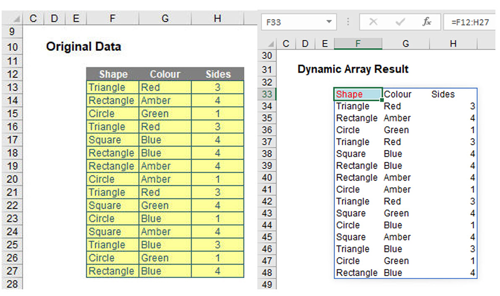
This is unprecedented behaviour for Excel. Instead of the formula having to be copied into every cell, the single formula in cell F33, known as a Spilled Array Formula, spills into F33:H48. But what happens if something is in the way, as shown in the screenshot below?

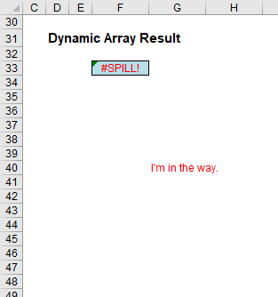
In this example, in cell G40, I have typed in the obtrusive text, “I’m in the way.” And it quite literally is. Consequently, I have generated the new #SPILL! error. The formula cannot spill, so the error message is generated accordingly.

The spiel on #SPILL! errors

#SPILL! errors are returned when a formula returns multiple results and Excel cannot return the results to the spreadsheet. There are various reasons a #SPILL! error could occur:

Spill range is not blank: As in my example above, this error occurs when one or more cells in the designated spill range are not blank and thus may not be populated.

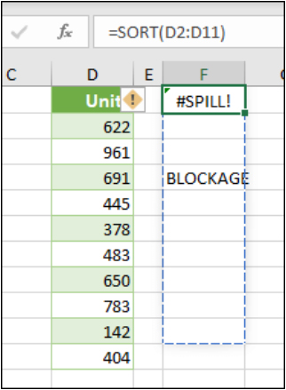
When the formula is selected, a dashed border will indicate the intended spill range. You may select the error “floatie” (believe it or not, this is what Microsoft calls these things), and choose the Select Obstructing Cell option to immediately go to the obstructing cell. You can then clear the error by either deleting or moving the obstructing cell’s entry. As soon as the obstruction is cleared, the array formula will spill as intended.

The range is volatile in size: This means the size is not “set” and can vary. Excel was unable to determine the spilled array’s size because it’s volatile and resizes between calculation passes. For example, the new function SEQUENCE(x) generates a list of x numbers increasing by 1 from 1 to x. That’s fine, but the following formula will trigger this #SPILL! error:

=SEQUENCE(RANDBETWEEN(1,1000))

Dynamic array resizes may trigger additional calculation passes to ensure the spreadsheet is fully calculated. If the size of the array continues to change during these additional passes and does not stabilise, Excel will resolve the dynamic array as #SPILL! This error type is generally associated with the use of RAND, RANDARRAY, and RANDBETWEEN functions. Other volatile functions such as OFFSET, INDIRECT, and TODAY do not return different values on every calculation pass and so tend not to generate this error.

The array extends beyond the worksheet’s edge: In this situation, the Spilled Array Formula you are attempting to enter will extend beyond the worksheet’s range. You should try again with a smaller range or array. For example, moving the following formula to cell A1 will resolve the error, and the formula will spill correctly:

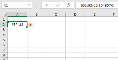
Table formula: As explained in the article “Excel: Arrays, Tables, and ‘The Twilight Zone’”, Tables and Dynamic Arrays are not yet best friends. Spilled Array Formulas aren’t supported in Excel Tables (generated by Ctrl+T). Try moving your formula out of the Table, or go to Table Tools > Convert to range.

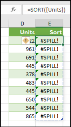
Out of memory: I have forgotten what this one means. Sorry, I couldn’t resist that. The Spilled Array Formula you are attempting to enter has caused Excel to run out of memory. Please try referencing a smaller array or range.

Spill into merged cells: Spilled Array Formulas cannot spill into merged cells. You will need to unmerge the cells in question or else move the formula to another range that doesn’t intersect with merged cells.

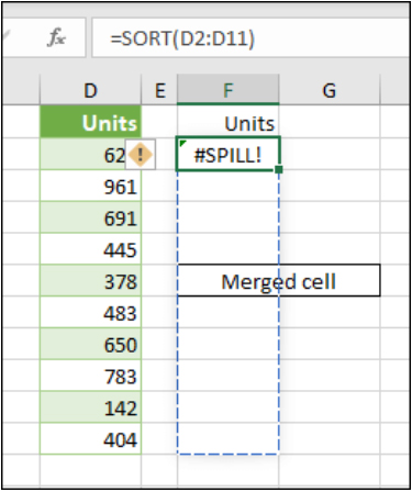
When the formula is selected, a dashed border will indicate the intended spill range. You can again select that wonderfully named error floatie and choose the Select Obstructing Cell option to immediately go to the obstructing cell. As soon as the merged cells are cleared, the array formula will spill as intended.

Unrecognised/fallback error: The catch-all variant. Excel doesn’t recognise, or cannot reconcile, the cause of this error. Here, you should make sure your formula contains all of the required arguments for your scenario.

Interlude: The #CALC! error

I mentioned there were two new error messages. I have only referred to #SPILL! so far. There is another, lurking in the background. (I say “in the background” because at the time of writing, Microsoft hasn’t written any documentation on it!).

Sometimes, as you explore how you can combine Excel functions with one another you get error messages (eg, more often than not trying FILTER(FILTER(… will generate a #VALUE! error). When you start playing with these new array functions, you might stumble upon #CALC! This is a new one.

To add to the myriad error messages such as #REF!, #DIV/0!, #VALUE!, #BROWN, and #PIPE, let’s introduce #CALC! — which probably means something like, “Excel cannot currently figure out the answer but might be able to in a future release — no promises, though.” I look forward to the documentation in due course though to fathom its real meaning (probably something like, “Help! Abandon ship!”).

Let’s move on.

Implicit intersection implications

The subhead for this section may be an alliteration and sound like something you can get arrested for, but Dynamic Arrays do come at a price. Not many users out there used the old method of doing arrays, but some did — and hence some legacy calculations will be affected.

In the past, if you entered =A$1:A$10 anywhere in rows 1 through 10, the formula would return only the value from that row. In fact, a spreadsheet our company is presently auditing relies on this behaviour. However, in the brave new world of Office 365 (albeit limited to selected Insider recipients for the time being), typing this formula would create a Spilled Array Formula. (A Dynamic Array Formula can produce multiple results in the future; a Spilled Array Formula has already produced multiple results, i.e., it has spilled.) To protect existing formulas, we need a new — if not instantly breathtaking — function.

SINGLE Function

Of the seven new Excel functions related to Dynamic Arrays, this one won’t set the world alight, but it is essential to keep Excel running smoothly. It’s like a toilet roll — imagine your situation without it.

The SINGLE function returns a single value using logic known as implicit intersection. SINGLE may return a value, single cell range, or an error.

The function has the following syntax:

=SINGLE(value)

The function has just one argument:

• value: this argument is required and represents the array to be selected.

When the supplied argument is a range, SINGLE will return the cell at the intersection of the row or column of the formula cell. Where there is no intersection, or more than one cell falls in the intersection, then SINGLE will return a #VALUE! error. When the supplied argument is an array, SINGLE returns the first item (Row 1, Column 1).

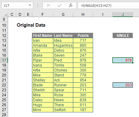
In the example below, the two SINGLE formulae (in cells J17 and J22) are supplied a range, H13:H27, and return the values in cells H17 and H22, respectively.

I can see an argument going forward that some form of OFFSET (eg, “NEXT” or “PRIOR”) may be needed in due course, but no one is expecting everything to come together on day 1.

So what’s next in our exploration of Excel’s evolution? A fun-filled journey through the six new functions that should have you excited. The navigation below will be updated with the article links once they go live.

An Excel Evolution: The Series

Getting started

Part 1: Excel: Microsoft Unveils Dynamic Upgrades

Part 2: Excel: Arrays, Tables, and ‘The Twilight Zone’

Part 3: Excel: 2 New Errors and a SINGLE Function

Function focus

Part 4: This Excel Change is More Than SORT of a Big Deal

Part 5: Focus on 2 New Excel Functions: UNIQUE and FILTER

Part 6: Excel New Function Focus: SEQUENCE and RANDARRAY

Final thoughts

Part 7: Will Dynamic Arrays Kill Data Tables, PivotTables?

— Liam Bastick, FCMA, CGMA, FCA, is director of SumProduct, a global consultancy specialising in Excel training. He is also an Excel MVP (as appointed by Microsoft) and author of An Introduction to Financial Modelling. Send ideas for future Excel-related articles to him at liam.bastick@sumproduct.com. To comment on this article or to suggest an idea for another article, contact Jeff Drew, an FM magazine senior editor, at Jeff.Drew@aicpa-cima.com.