Functional beauty: Laying out a proper Excel model

Most spreadsheets serve a purpose, typically to communicate a forecast, evaluate a project, or undertake some other form of quantitative analysis. Note the verb communicate. Spreadsheets are communicative tools first and foremost. However, that communication is frequently sullied by poor layouts, insufficient labels, and inconsistencies that cause end users difficulties in understanding the model’s purpose and content. These issues can lead to unnecessary extra work for the model-builder, make it difficult for the decision-maker to understand, and result in conclusions based upon errors in logic and/or formulas that are not readily identifiable or visible.

Therefore, you should put some thought into designing your spreadsheets and not just the formulas, functions, and formats you use. That is the focus of this month’s column, which builds upon the Best Practice modelling principles described in my March article “How to Craft the Best Excel Spreadsheet Models”. As you may recall, I capitalise Best Practice to emphasise that it is in this usage a proper noun reflecting the idea that a good model has four key attributes I call CRaFT:

• Consistency;
• Robustness;
• Flexibility; and
• Transparency.

With this in mind, let me explain how I think when putting a worksheet together:

Building an effective communication tool by laying out an appropriate financial model is simple: It’s all about designing and scoping. The problem is, we are all time-poor in today’s business environment with perpetual pressure to produce results quickly. Getting a layout structure won’t solve all your problems, but it’s a start.

Let me show you how I develop a basic worksheet, starting with a blank worksheet. Assuming this isn’t a dashboard output page where column width may be more critical, I tend to narrow the first few columns (highlight columns, then right-click and select Column width … from the pop-up context menu):

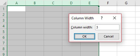
It may not be clear why I choose to do this, but read on (hey, I need to keep you on the edge of your seat!). I choose a width of 3, which effectively makes the cells in these columns square.

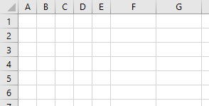
You can highlight a different number of columns, and you can modify the width used, too. There are two key points to this:

1. Keep column A blank other than for the sheet headings, which I will explain later.
2. Be consistent, both with the width of the columns narrowed here and with other worksheets in the same workbook. Again, I will explain soon.

Next, let’s put the sheet title in cell A1. This should be the same as the description in the sheet tab. For this example, I named it “Sheet Title” to emphasise the purpose of this placeholder, but without the quotation marks:

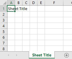
There are three reasons for this:

1. Given that sheet tab names cannot be infinitely long, “Sheet Title” is more succinct and easier for the end user to understand.
2. Given that the sheet title appears on the worksheet, the name has to be written formally and cannot be an incomprehensible abbreviation.
3. This approach promotes consistency, one of the four key concepts of Best Practice modelling.

In cell A2, I put the model name. This is important as often we show only extracts of a workbook in an appendix to a report or a PowerPoint presentation. Therefore, I place it here rather than in the header or footer of each worksheet instead (but you may do both):

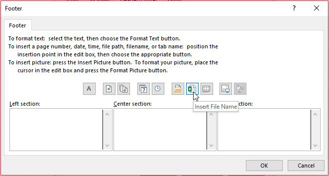
If you intend to add this to the header or footer, these attributes may be accessed by the keyboard shortcut ALT + P + SP -> ‘Header / Footer’ tab -> ‘Custom Footer…’ button. I acknowledge it’s simpler than my alternative, but this filename will display only when the worksheet is printed. What if it is an image on a PowerPoint slide or, say, as Appendix 4 in a Word document? This is why I keep the model name front and centre on my worksheets.

There’s a formula, too:

=IFERROR(MID(CELL("filename",A1),FIND("[",CELL("filename",A1))+1,FIND("]",CELL("filename",A1))-FIND("[",CELL("filename",A1))-1),"")

To see how a similar formula was derived, please see my April article, “Automating in Excel: A Worksheet Display Tip”.

The next key item to position at the top is a navigation aid. Today’s workbooks can be quite complex with many worksheets. I recommend incorporating a central navigation page — a “Table of Contents” — that allows the end user to traverse the workbook quickly and easily.

It looks as if I have added a hyperlink in cell A3, right? Actually, I have highlighted cells A3:F3 and then merged the cells using Excel’s Merge Across functionality (ALT + H + M + A):

Hyperlinks may be created easily using the keyboard shortcut CTRL + K (or by clicking the Link button on the Insert tab) to link to a place in your document. The intention is to set up a central Table of Contents worksheet where all the hyperlinks to the other worksheets reside:

The hyperlink should link to cell A1 of that worksheet, and that cell should have a range name such as HL_TOC. A range name is essential to avoid a broken link should someone rename the destination worksheet. “HL” denotes that the cell is used as the destination for a hyperlink. The cells A3:F3 are merged so that if the end user clicks anywhere in that range, the hyperlink will activate; otherwise, the user would have to click on cell A3 for the hyperlink to work.

This brings us on nicely to cell A4:

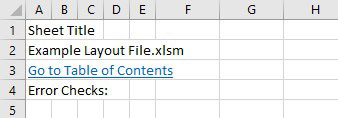
We can add a formula here to summarise any error checks present in the model. Typically, to conserve real estate on the worksheet, dates and other headings may share this row, too:

In my layout, column G is the Units column. Down this column I shall put in all my units so end users may distinguish between numerical fields. How often have you seen a printout and not known if it is in $, $’000, $m, kg, or sliced tomatoes? This will make this issue a thing of the past. It should be noted that this column is not always required. For instance, on an outputs worksheet, you may simply state near the top of the sheet, “All outputs are displayed in $m unless stated otherwise”.

Cells J4:N4 contain the date headings. The dates should be periodic (eg, monthly, quarterly, annually) and should always start and end in the same columns (and rows) on each forecast worksheet. That is not always possible: Sometimes, you require some of your model to be annually forecast and other aspects monthly. Where different reporting periodicities are necessary, these inconsistent worksheets should be clearly delineated from other areas of the workbook.

You may have noticed there appears to be a line inserted between rows 4 and 5 of the image:

This is not a drawn line. This is called a frozen pane. Frozen panes break up the worksheet into as many as four pieces and allow parts of the worksheet to remain on view (“be frozen”) whilst the reader scrolls down or across the worksheet. In the Window grouping of the View tab of the ribbon, Excel provides three ways to create a frozen pane:

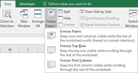
• Freeze Top Row: This keeps the top row visible no matter how far down the spreadsheet you scroll.
• Freeze First Column: This keeps the first column visible no matter how far to the right you scroll the spreadsheet.
• Custom (Freeze Panes): This creates a frozen locus at the intersection of the top row and the first column of the cell(s) selected.

That final option is a little confusing. Essentially, the frozen panes are created as follows:

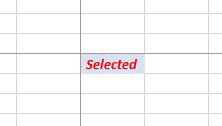
Frozen panes are created for the region the selection is in, the region directly above, the region to the immediate left, and diagonally opposite the top left corner of the selection. If the selection were in column A, there would be only two frozen panes: the rows immediately above and the rest of the sheet. If the selection were in row 1, again, there would be only two frozen panes: the columns to the left and the remainder.

In this example, cell A5 has been made the basis of the frozen pane, so that rows 1 to 4 will always be visible. This cell should be given a range name, eg, HL_Home, as this is the cell to which hyperlinks to this sheet should link. This cell “resets” the sheet when a frozen pane has been added (not cell A1) and makes the model easier to navigate consequently. This cell can be identified by employing the keyboard shortcut CTRL + HOME.

Now, let me explain the unexplained narrowing of the first few columns. I would suggest headings should start in column B, not A, and then move out a column or two for subheadings and sub-subheadings, respectively. This causes a natural indentation. I then put data labels directly beneath sub-subheadings:

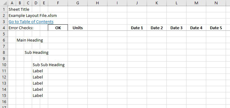
I have called them “headings”, “subheadings”, etc., to make it clear, but this approach will become cumbersome quickly. Renaming as Heading 1 and Heading 2 is clearer. This also makes them consistent with pre-existing Style names (hint, hint):

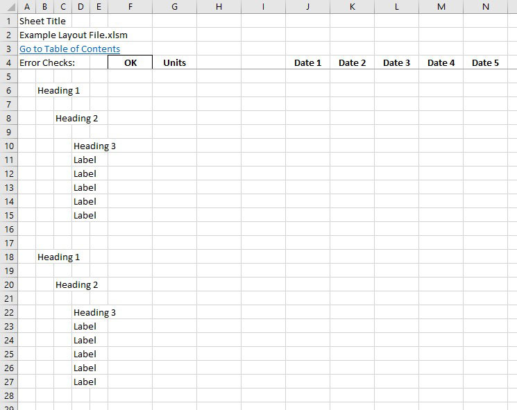
Aside from keeping column A clear, do you now see why I have narrowed columns B, C, and D (I am keeping column E “just in case”)? The narrowing of the columns effectively indents the headings and makes worksheets easier to read and navigate (especially if the gridlines, ALT + W + VG, are toggled off).

Take note of the spacing: one blank row between headings; two lines between sections. That’s my preference. You may choose your own if you prefer — just be consistent. It makes it simple to copy sections and keep referencing if spacing is deliberate.

Blank columns H and I are in existence in case we have any calculations, inputs, or referred values that do not refer to a particular time period. If they are not required, I tend to narrow the columns to a width of 1, so that they are still there in case they are needed later.

Adding labels, data, and formulas:

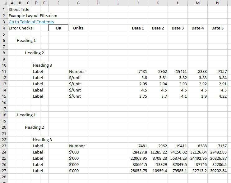
It’s starting to look more like a spreadsheet now. The next step is to incorporate Styles (ALT + H + J), as shown below:

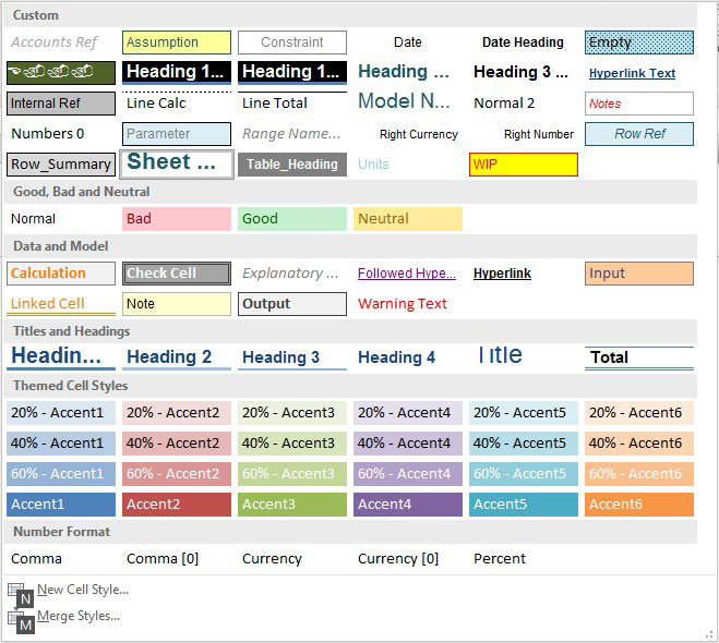
Very quickly, our spreadsheet is taking shape:

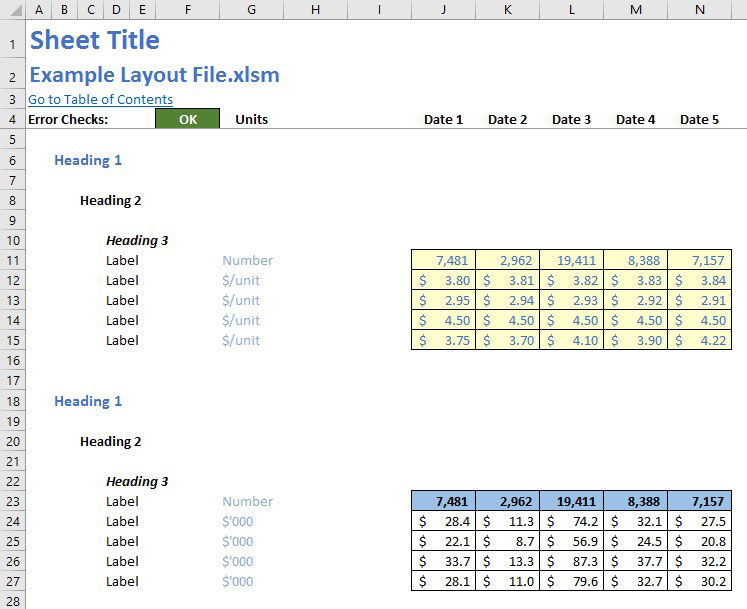
If I switch off gridlines on my spreadsheets, then most of my files appear to have a white background. There is more to this point than merely aesthetics. Adding a colour to the background of a spreadsheet can make a file significantly larger — unnecessarily.

The spacing is deliberate, too. Not only does it look neater (remember, Excel 2007 onwards has 1,048,576 rows and 16,384 columns, ie, it is 1,024 times larger than an Excel 2003 worksheet, so there is plenty of room), but the space is functional, too.

Want to navigate between the main headings in column B? Click on cell B6, go CTRL + Down Arrow, and you will arrive at cell B18. Repeat this action, and the next cell you will hit is cell B1048576, ie, the very bottom of the spreadsheet because there is nothing else in this column.

Click on cell D10 (Heading 3) and use the keyboard shortcut CTRL + Down Arrow to take you to cell D15, the final cell in the contiguous range. CTRL + Up Arrow, CTRL + Right Arrow, and CTRL + Left Arrow will all perform similar actions. Need to highlight a range? Click on any cell within the range and CTRL + A will select the whole contiguous range. This makes the model easier for developer and user alike to navigate and manipulate.

So why have I kept column A blank? The reason is to take into account work in progress. How often have you started creating a spreadsheet only to be interrupted, have to go to a meeting, take a telephone call, go home, or go to sleep? The point is, when we are interrupted, we need to remember how far along we were. If you design a spreadsheet similar to the one discussed here, imagine you are interrupted without notice. Before you turn your attention to the disruption, whichever row you are working on, press the HOME key, which will take you to column A of that row. Type anything in that cell, eg, “w” for “work in progress” or “check” and so on. That’s it.

Word to the wise

Whatever you decide to do, keep it consistent, make it transparent, and ensure there are checks to protect the robustness and that inputs are clearly marked to aid flexibility. Any layout addressing these points will necessarily adhere to the CRaFT ideology.

— Liam Bastick, FCMA, CGMA, FCA, is director of SumProduct, a global consultancy specialising in Excel training. Send ideas for future Excel-related articles to him at liam.bastick@sumproduct.com. To comment on this article or to suggest an idea for another article, contact Jeff Drew, an FM magazine senior editor, at Jeff.Drew@aicpa-cima.com.