How to use Excel for practical debt repayment calculations

The start of a new year is a time for planning, renewal, and figuring out how to pay off that holiday debt. This article considers how to model debt repayment calculations from a practical perspective. It addresses three common calculations using Excel’s financial functions for the last item.

For completeness, my examples include the seemingly more convoluted mathematical formulas that arrive at the same answer. This is because some of the useful functions (eg, CUMPRINC) are not in the “basic” Excel function directory for some versions of Excel. The mathematical alternatives work without relying upon this add-in using no more than the standard operators plus the LOG function on occasion.

For simplicity, the discussion below focuses on scenarios where payments are made at the end of each period (ie, payments are “in arrears”). All of the following examples are considered further (including when payments are made “in advance”) in the attached Excel file.

Problem 1: Minimum payment calculations (PAiN relief)

This is often referred to as the mortgage calculator. Here, the aim is to calculate what the regular repayment is per period to service and pay off a debt over a given amount of time.

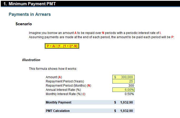
For example, if I borrow $300,000 over 25 years at an interest rate of 6% per annum, what will my regular monthly payments be (assuming no change of rate)?

The answer is given by the formula:

P = Ai / (1 – (1 + i)^-N) where:

• P = regular periodic payment
• A = amount borrowed
• i = periodic interest rate
• N = total number of repayment periods

(It’s interesting that the acronym for remembering the mortgage variables is PAiN!)

In our example, crunching the numbers (using a periodic interest rate of 0.50%, which is 6% ÷ 12 months, and total number of periods being 25 × 12 = 300) gives a monthly repayment of $1,932.90.

The same calculation could have been performed in seconds using Excel’s built-in PMT function:

PMT (rate,number_of_periods,amount_of_loan)

It should be noted that using PMT will give the same solution but be negative instead. This is because Excel’s financial functions distinguish between cash inflows (positive) and outflows (negative).

Problem 2: Calculating the outstanding balance

If we want to refinance or pay off a loan, we need to be able to forecast the balance outstanding at a point of time (ignoring penalties, etc.).

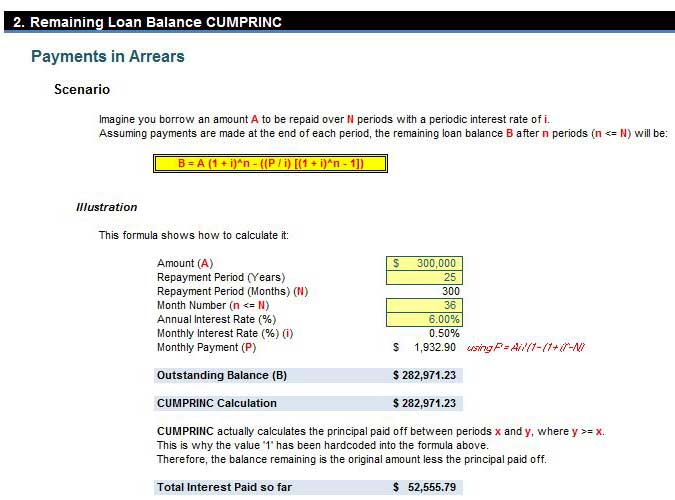
Continuing the example from above, I have borrowed $300,000 over 25 years at an interest rate of 6% and am making monthly (minimum) repayments. After three years, I am able to refinance my loan without incurring any penalties. What would be the outstanding amount at this point in time?

The answer to this question is given by the formula:

B = A(1 + i)ⁿ – (P((1 + i)ⁿ - 1) / i) where:

• B = balance outstanding
• P = regular periodic payment
• A = amount borrowed
• i = periodic interest rate
• n = number of periods payments that have been made (n <= N)

Using the same periodic interest rate of 0.50%, the monthly repayment of $1,932.90 (calculated above) and using 36 (12 × 3) periods for n, the amount outstanding would be $282,971.23, ie, only $17,028.77 (principal) has been paid off. If we calculate the total of the payments made (36 × $1,932.90), then the inferred interest is a whopping $52,555.79! Best not to think too long about it.

The same calculation could have been performed quickly using Excel’s CUMPRINC function:

CUMPRINC(rate,life_of_loan,amount_of_loan,start_period,end_period,type)

This requires explanatory notes:

• Again, the rate is the periodic rate (here 0.50%, not 6%).
• life_of_loan is the total length of the loan, not just to date. This is needed to calculate implicitly the regular repayment amount.
• CUMPRINC actually calculates the amount of principal paid off for an interval of time (CUMPRINC = cumulative principal). Therefore, the start and end dates must be stipulated, and if we are calculating the aggregate from the beginning, the start_date must be 1 (first period).
• The type determines whether payments are made in arrears (type 0) or in advance (type 1).
• To calculate the balance outstanding using this method, we simply compute Amount + CUMPRINC calculation.

It should be noted that, similar to PMT, CUMPRINC gives a negative value for similar reasons. This is why the formula employs addition rather than subtraction.

Problem 3: How long before the debt is paid off?

What if we decide to turn the problem around? Instead of determining the amount outstanding, how do we calculate how long a debt will take to pay off if we decide to stipulate what the regular payment will be each month instead?

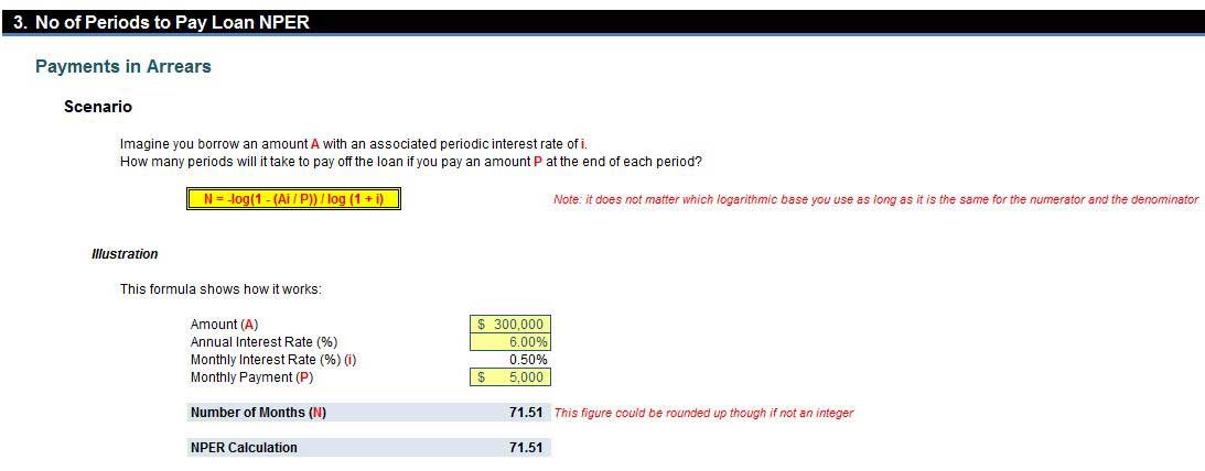
Returning to my example, if I borrow $300,000 at an interest rate of 6%, how long will it take to pay off if I pay $5,000 each month? This assumes that our payment exceeds the accrued interest each month (here, $300,000 × 0.50% = $1,500).

The answer is given by the formula:

N = -log(1 – (Ai / P)) / log (1 + i) where:

• N = total number of repayment periods
• A = amount borrowed
• i = periodic interest rate
• P = regular periodic payment

(The logarithmic base is irrelevant as long as the same one is used for the numerator and denominator of the above quotient.)

Plugging the inputs into the formula gives us a value of 71.51, ie, 72 periods (fractions of periods do not really make sense here).

The same calculation could have been computed simply using the NPER function:

NPER(rate,-payment,amount_of_loan)

Note that the payment must be negative, and the amount of the loan must be positive. 

Word to the wise

There are several other functions that can answer questions posed by modifying our scenarios above. Common functions include PPMT (amount of principal paid in a given period of time), IPMT (amount of interest paid in a given period of time [note PPMT + IPMT = PMT for any one period]), and RATE (the implied interest rate for an annuity). However, with the exception of RATE (where Goal Seek is often used instead), these other functions can often be circumvented using extensions of ideas illustrated in the examples above.

As with many things in Excel, there is more than one approach to the correct answer.

Liam Bastick is director of SumProduct, a global consultancy specialising in Excel training. Send ideas for future Excel-related articles to him at liam.bastick@sumproduct.com. To comment on this article or to suggest an idea for another article, contact Neil Amato, an FM magazine senior editor, at Neil.Amato@aicpa-cima.com.