This Excel change is more than SORT of a big deal

Editor’s note: Microsoft recently announced a partial rewrite of Excel’s calculation engine. The result is an evolutionary leap that promises to bring numerous improvements to Excel users in the coming years. Already unveiled are a new type of calculation (Dynamic Arrays), seven new functions, and two new errors. These changes have not yet been rolled out to all Excel users, but you don’t have to wait to see what they can do. Excel MVP Liam Bastick is covering all the changes in a seven-part series. In this instalment, Bastick walks you through two of the new functions — SORT and SORTBY. 

If you haven’t read the first three articles in this series, you really should. Just click on one of the links below:

• Part 1: Excel: Microsoft Unveils Dynamic Upgrades
• Part 2: Excel: Arrays, Tables, and ‘The Twilight Zone’
• Part 3: Excel: 2 New Errors and a SINGLE Function

On the off-chance you are new to this series and don’t have the time or inclination to read the first three articles, here’s a (relatively) brief summary. Microsoft’s new Dynamic Arrays functionality greatly simplifies the process of working with arrays in Excel. There’s no more copying formulas to the entire range and having to press Ctrl+Shift+Enter to see multiple results. Instead, you enter a formula in one cell, and, poof, the data you are looking for just spill out. Look at the screenshots below. As you can see, the formula entered into cell F33 in the right image is =F12:H27, which references the original data shown in the left image.

As you can see, the formula spills (ie, it automatically extends into the designated area — in this case, three columns by 16 rows.). This type of formula is called a Spilled Array Formula, and Excel has introduced seven new functions that work with Spilled Array Formulas. One of the new functions, SINGLE, is needed to make workbooks with the old array formulas work with the updated Excel calculation engine (see “Excel: 2 New Errors and a SINGLE Function”). As for the other arrays, let’s go through them in an order that makes sense (well, to me anyway).

Function focus: SORT

Our first function is one people have been crying out for — for years. Enterprising spreadsheet gurus have developed array formulas and user-defined functions that have replicated the functionality of the new SORT function, but those won’t be needed once Microsoft makes SORT generally available.

So what’s the big deal? Let’s start with the syntax. The SORT function sorts the contents of a range or array, as follows:

=SORT(array, [sort_index], [sort_order], [by_column]).

It has four arguments:

• array: this is required and represents the range that is required to be sorted.
• sort_index: this is optional and refers to the position of the row or the column in the selected array (eg, second row, third column). About 98 times out of 99 you will be defining the column, but to select a row you will need to use this argument in conjunction with the fourth argument, by_column. And be careful, it’s a little counterintuitive! The default value is 1.
• sort_order: this is also optional. The choices for sort_order are either 1 for ascending (default) or -1 for descending. It should be noted that you might not want to hold your breath waiting for sort by colour, formula, or custom list using this function.
• by_column: this final argument is also optional. Most people want to sort rows of data, so they will want the value to be FALSE (which is the default value if not specified).

To show you how devilishly simple it is, consider the following data:

Sorting the “Points” column in order is easy. All you have to do is type =SORT(H13:H27) into cell F32.

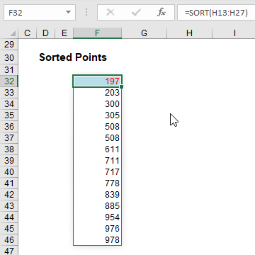
Simple, right? Note that the duplicates are repeated; there is no cull. If you want it in descending order, the formula is only slightly more sophisticated, in that the sort_order (third argument) needs to be specified as -1 to switch the sort to descending:

=SORT(H13:H27,,-1).

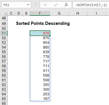
Again, simple. But, you might be asking, why would anyone want to list the points all by themselves? What about the names?

Great questions, and the answer is that this is where all of these arguments in the SORT formula start to make more sense. Consider the screenshot below. SORT(F13:H27,3,-1) produces the whole array (array is F13:H27), sorts it on the third (sort_index 3) column in descending (sort_order -1) order. Blake and Ivana tie on 508 points, but Blake appears first as he was first in the original (source) table.

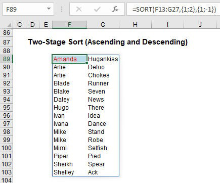
So far, I have performed only one SORT. You can have more than one though. In the screenshot below, I have created a second (two-level) SORT. Here, you need to create what is known as an array constant for the second and third arguments (you just type the braces in — don’t use Ctrl+Shift+Enter):

=SORT(F13:G27,{1;2},{1;-1}).

This formula will sort on column 1 (“First Name”) first, then sort on column 2 (“Last Name”). This will be in ascending order (1) for the first column and descending order (-1) for the latter. It’s not as straightforward a formula entry as most Excel modellers are used to, but it’s relatively straightforward once you have committed it to memory.

My final example of SORT is not something that is limited to this new function, but it does show how things fit together. From the first three articles in this series, it might appear you can only get one value (using SINGLE) or all of them (using Dynamic Arrays). That’s not true as this illustration clearly demonstrates:

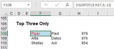
Only the top three have spilled in this example. How? Well, I cheated. I highlighted cells F108:H110 first, then typed in the formula:

=SORT(F13:H27,3,-1)

and then pressed Ctrl+Shift+Enter (thus generating the { and } braces). This restricted the spill to the range stipulated. Cool. Other than making sure no one can delete or insert any rows by creating an array formula such as {=1} across the restricted area, these appear to be the only two uses of Ctrl+Shift+Enter now.

SORT is really useful then, but what if you want to sort on a field you don’t want displayed in the results?

Function focus: SORTBY

The SORTBY function sorts the contents of a range or array based on the values in a corresponding range or array, which does not need to be displayed. The syntax is as follows:

=SORTBY(array, by_array1, [sort_order1], [by_array2], [sort_order2], …).

It has several arguments:

• array: this is required and represents the range that is required to be sorted.
• by_array1: this is the first range that array will be sorted on and is required.
• sort_order1, sort_order2, …: these are optional. The choices for each sort_order are 1 for ascending (default) or -1 for descending.
• by_array2, …: these arguments are also optional. These represent the second and subsequent ranges that array will be sorted on.

There are some important considerations to note:

• the by_array arguments must either be one row high or one column wide.
• all of the by_array arguments must be the same size and contain the same number of rows as array if sorting on rows, or the same number of columns as array if sorting on columns.
• if the sort order argument is not 1 or -1, the formula will result in a #VALUE! error.

It’s pretty simple to use. Consider the following source data once more:

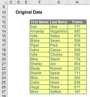
I can use SORTBY using the formula: =SORTBY(F13:F27,H13:H27,-1,G13:G27,1). This produces the results shown in the screenshot below.

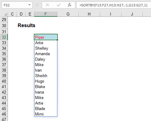
Note that I have sorted the “First Name” field (F13:F27) on the “Points” column (H13:H27) in descending (-1) order and then used the second sort on “Last Name” (G13:G27) in ascending (1) order. No need for those pesky array references in multiple sorts with the SORT function (as detailed above).

An Excel Evolution: The Series

Getting started

Part 1: Excel: Microsoft Unveils Dynamic Upgrades

Part 2: Excel: Arrays, Tables, and ‘The Twilight Zone’

Part 3: Excel: 2 New Errors and a SINGLE Function

Function focus

Part 4: This Excel Change is More Than SORT of a Big Deal

Part 5: Focus on 2 New Excel Functions: UNIQUE and FILTER

Part 6: Excel New Function Focus: SEQUENCE and RANDARRAY

Final thoughts

Part 7: Will Dynamic Arrays Kill Data Tables, PivotTables?

— Liam Bastick, FCMA, CGMA, FCA, is director of SumProduct, a global consultancy specialising in Excel training. He is also an Excel MVP (as appointed by Microsoft) and author of An Introduction to Financial Modelling. Send ideas for future Excel-related articles to him at liam.bastick@sumproduct.com. To comment on this article or to suggest an idea for another article, contact Jeff Drew, an FM magazine senior editor, at Jeff.Drew@aicpa-cima.com.