Focus on 2 new Excel functions: UNIQUE and FILTER

Editor’s note: Microsoft recently announced a partial rewrite of Excel’s calculation engine. The result is an evolutionary leap that promises to bring numerous improvements to Excel users in the coming years. Already unveiled are a new type of calculation (Dynamic Arrays), seven new functions, and two new errors. These changes have not yet been rolled out to all Excel users, but you don’t have to wait to see what they can do. Excel MVP Liam Bastick is covering all the changes in a seven-part series. In this instalment, Bastick shows how to use two of the new functions, FILTER and UNIQUE.  

In Part 4 of this series, we covered arguably the two most exciting of the seven fresh functions that work with Excel’s new Dynamic Arrays capabilities. You don’t have to read Part 4 before reading this article, but it’s worth checking out (you should find it at least SORT of helpful).

If you haven’t read Parts 1–3, don’t despair! If you want to catch up, the links are at the bottom of this article. If you don’t want to read three articles before continuing this one, the following section covers what you need to know about Dynamic Arrays (if you have read the other articles, you can jump ahead to the “Fiddling With the FILTER Function” section).

Dynamic Arrays: A quick review

Microsoft’s new Dynamic Arrays functionality greatly simplifies the process of working with arrays in Excel. There’s no more copying formulas to the entire range and having to press Ctrl+Shift+Enter to see multiple results. Instead, you enter a formula in one cell and, poof, the data you are looking for just spill out. Just look at the screenshots below. As you can see, the formula entered into cell F33 in the right image is =F12:H27, which references the original data shown in the left image.

The functionality shown above is unprecedented in Excel. Of the seven new functions that come with Dynamic Arrays, the two covered in this article are interesting on their own but combine them with other functions and good things start to happen, as shown with the SORT(UNIQUE(FILTER())) formula mentioned later in the article. But first ...

Fiddling with the FILTER function

The FILTER function will accept an array, allow you to filter a range of data based upon criteria you define, and return the results to a spill range.

The syntax of FILTER is as follows:

=FILTER(array, include, [if_empty]).

It has three arguments:

• array: This is required and represents the range that is to be filtered.
• include: This is also required. This specifies the condition(s) that must be met.
• if_empty: This argument is optional. This is what will be returned if no data meets the criterion/criteria specified in the include argument. It’s generally a good idea to at least use "" (ie, a pair of double quotation marks) here.

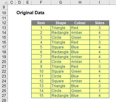
For example, consider the following source data:

To begin with, I will perform a simple FILTER:

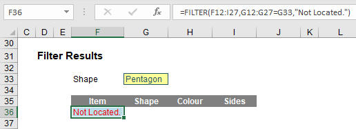
Here, in cell F36, I have created the formula

=FILTER(F12:I27,G12:G27=G33,"Not Located.")

F12:I27 is my source array and I wish only to include shapes (column G12:G27) that are Triangles (specified by cell G33). If there are no such shapes, then “Not Located.” is returned instead. To show this, I will change the shape as follows:

That is about as basic as it gets. I can get cleverer. Consider the following example:

I have repeated the source array (cells F48:I63) for clarity. The formula

=FILTER(F48:I63,(G48:G63=G69)*(H48:H63=G70),{"-","None","N/A","N/A"})

looks horrible to begin with, but it’s not quite as bad as it appears upon further scrutiny. The argument below,

(G48:G63=G69)*(H48:H63=G70)

contains two conditions. Firstly, G48:G63=G69 means that the “Shape” (column G48:G63) has to be a “Triangle” (cell G69) and that the “Colour” (column H48:H63) has to be “Red” (cell G70). The multiplication operator (*) is used to denote AND. The Excel function AND cannot be used with arrays — this is nothing special to Dynamic Arrays; AND does not work with Ctrl+Shift+Enter formulas either. This syntax is similar to how you would create AND criteria with the SUMPRODUCT function, for example.

The final argument is similar to the syntax in SORT: {"-","None","N/A","N/A"}. Braces (typed in!) are used to create an array argument that specifies what should be written in each column should there be no record that meets both criteria, eg.

See? Not as bad as you might first think.

My final example is very similar:

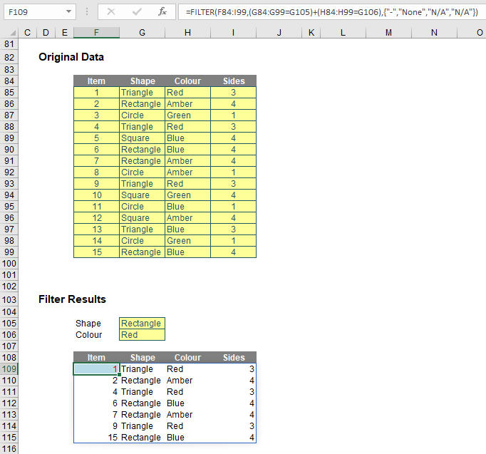
Once you realise I have simply repeated referencing for clarity, the formula

=FILTER(F84:I99,(G84:G99=G105)+(H84:H99=G106),{"-","None","N/A","N/A"})

is nothing more than the OR equivalent of the previous example, with + replacing * to switch from ensuring both conditions are met to only one condition being met. As at the time of writing, XOR is not catered for, but I am sure some clever person will create an equivalent in due course (if Microsoft doesn’t beat them to it), necessity being the mother of invention and all that jazz.

This function takes a UNIQUE approach

The hilarious thing about UNIQUE is that it does two things. It details distinct items (ie, provides each value that occurs with no repetition), and it also can return values that occur once and only once in a referred range. I understand that Excel users may welcome the former use with open arms and that database developers may be very interested in the latter. I still think there should have been two functions though. Otherwise, let’s just extend the AGGREGATE function to do just everything (it almost does now) and be done with it!

The UNIQUE function has the following syntax:

=UNIQUE(array, [by_column], [occurs_once]).

It has three arguments:

• array: This is required and represents the range or array from which to return unique values.
• by_column: This argument is optional. This is a logical value (TRUE/FALSE) indicating how to compare. If you wish to compare by row, the argument should be FALSE or omitted (since this is the default). To compare by column, you will need to select TRUE.
• occurs_once: This argument is also optional. This requires a logical value, too:
  • TRUE: Return only unique values that occur once;
  • FALSE: Include all distinct values (default if omitted).

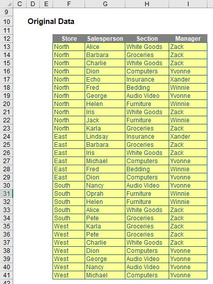
It’s probably clearer with some examples. Let’s give it a go. As always, I need source data:

Time for the most basic illustration:

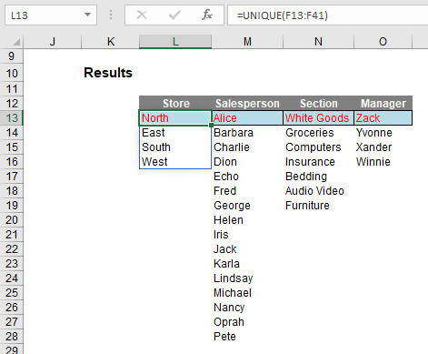
In cell L13, I have simply typed

=UNIQUE(F13:F41).

No optional arguments; everything in default. If I have made an error, it’s going to be my default. This has simply listed each store that appears; if “North” and “North ” (extra space) were there, then both would appear. UNIQUE is not case sensitive though, and each entry would appear as it first occurs reading down the range F13:F41. The other columns contain similar formulas, and UNIQUE looks like it takes seconds to learn.

It’s just as simple if you want to see unique records for two (or more) columns, as shown in the screenshot below.

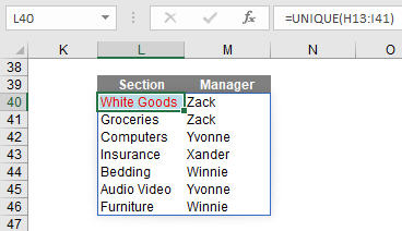
You can see UNIQUE is sort of crying out for SORT, but we’ll get to that shortly.

As mentioned earlier, it’s not the only way of using UNIQUE (no, having a unique use would be just what “they” were expecting, whoever “they” are …). You can use it to determine values that occur only once:

Here, the formula in cell L56,

=UNIQUE(G56:G84,0,1)

uses the nondefault value of 1 for the optional occurs_once (third) argument. This means it identifies the salespeople who occur only once in cells G56:G84. Brilliant! I can die content now.

The real power starts coming when you start playing with Excel’s existing functions and features, together with these new functions. Take this comprehensive example:

Let me step you through some of this. The formulas in cells L94 and M94 use UNIQUE in a similar manner to my first example, to generate the list of distinct values in the “Section” and “Manager” fields. However, did you notice they have been sorted? That’s because I used the formula

=SORT(UNIQUE(H94:H122))

in cell L94, for example. Honestly, I think UNIQUE should have another argument for sorting (ascending/descending/none [default]). Watch Microsoft ignore that suggestion.

But then I did something really cool. Cells M105 and M106 use data validation (Alt+D+L) to generate a list from the “Lookup Data” section. That requires taking a closer look:

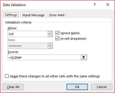
Do you see the source for the data validation in cell M105? =$L$94# — so elegant! This takes the “Section” list and automatically makes the dropdown list the required length! People create all sorts of tricks using OFFSET, dynamic range names, and the like to achieve a similar effect. No more. =$L$94# (with the #, the Spilled Range Operator) is all that is needed. That’s my favourite thing in all of these new functions and features. I’m impressed.

The AND/OR dropdown is a bit of an anticlimax after that, but the final formula that generates the final table, namely

=SORT(UNIQUE(FILTER(F93:I122,IF(M108="OR",(H93:H122=M105)+(I93:I122=M106),
(H93:H122=M105)*(I93:I122=M106)),{"N/A","-","-","-"})),{1;2;3;4},{1;1;1;1})

is rather fun. I am not going to go through it though — as every aspect of this formula is simply a rehash of an earlier point (assuming you know the IF function!). See if you can work your way through it for yourself.

An Excel Evolution: The Series

Getting started:

Part 1: Excel: Microsoft Unveils Dynamic Upgrades

Part 2: Excel: Arrays, Tables, and “The Twilight Zone”

Part 3: Excel: 2 New Errors and a SINGLE Function

Function focus:

Part 4: This Excel Change is More Than SORT of a Big Deal

Part 5: Focus on 2 New Excel Functions: UNIQUE and FILTER

Part 6: Excel New Function Focus: SEQUENCE and RANDARRAY

Final thoughts

Part 7: Will Dynamic Arrays Kill Data Tables, PivotTables?

— Liam Bastick, FCMA, CGMA, FCA, is director of SumProduct, a global consultancy specialising in Excel training. He is also an Excel MVP (as appointed by Microsoft) and author of Introduction to Financial Modelling. Send ideas for future Excel-related articles to him at liam.bastick@sumproduct.com. To comment on this article or to suggest an idea for another article, contact Jeff Drew, an FM magazine senior editor, at Jeff.Drew@aicpa-cima.com.