Excel new function focus: SEQUENCE and RANDARRAY

Editor’s note: Microsoft recently announced a partial rewrite of Excel’s calculation engine. This result is an evolutionary leap that promises to bring numerous improvements to Excel users in the coming years. Already unveiled are a new type of calculation (Dynamic Arrays), seven new functions, and two new errors. These changes have not yet been rolled out to all Excel users, but you don’t have to wait to see what they can do. Excel MVP Liam Bastick is covering all the changes in a seven-part series. In this instalment, he walks you through two of the new functions.

In Parts 1–5 of this series, we introduced Excel’s new Dynamic Arrays capabilities, showed how Dynamic Arrays work, covered two new errors (for when Dynamic Arrays don’t work), and examined five of the seven new functions that come with Excel’s arrays-ing new tool.

This article features the final two stops on the function(al) phase of our journey. If you haven’t read any of the first five parts, you are encouraged to do so. Links are available at the bottom of the article. If you want to press forward, here’s a quick review of what Dynamic Arrays are and how they work.

Dynamic Arrays: A quick review

Microsoft’s new Dynamic Arrays functionality greatly simplifies the process of working with arrays in Excel. There’s no more copying formulas to the entire range and having to press Ctrl+Shift+Enter to see multiple results. Instead, you enter a formula in one cell and, poof, the data you are looking for just spill out. Just look at the screenshots below. As you can see, the formula entered into cell F33 in the right image is =F12:H27, which references the original data shown in the left image.

As already mentioned, Microsoft has created seven new functions to work with the new Dynamic Arrays capabilities. As is the case with the functions covered in Part 5 of this series, the functions focused on in this article, SEQUENCE and RANDARRAY, really come to life when combined with other functions, as illustrated below.

Going through SEQUENCE step by step

The penultimate function in this series is SEQUENCE. This function allows you to generate a list of sequential numbers in an array, such as 1, 2, 3, 4. It doesn’t sound particularly exciting, but it really ramps up when combined with other functions and features. The syntax is given by:

=SEQUENCE(rows, [columns], [start], [step]).

It has four arguments:

• rows: This argument is required and specifies how many rows the results should spill over.
• columns: This argument is optional and specifies how many columns (surprise, surprise) the results should spill over. If omitted, the default value is 1.
• start: This argument is also optional. This specifies what number the SEQUENCE should start from. If omitted, the default value is 1.
• step: This final argument is also optional. This specifies the amount each number in the SEQUENCE should increase (the “step”). It may be positive, negative, or zero. If omitted, the default value is 937,444. Wait, I’m kidding; it’s 1. They’re very unimaginative over in Redmond.

Therefore, SEQUENCE can be as simple as SEQUENCE(x), which will generate a list of numbers in a column 1, 2, 3, …, x. Therefore, be mindful not to create a formula where x may be volatile and generate alternative values each time it is calculated, eg, =SEQUENCE(RANDBETWEEN(10,99)) as this will generate a #SPILL error because the range is volatile in size.

A vanilla example is rather bland:

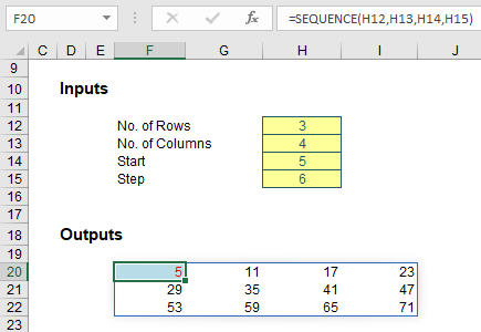
Do you see how SEQUENCE propagates across the row first and then down to the next row, just like reading a book? I wonder how that might work in alternative languages of Excel where users read right to left. (It has to be the same or there would be chaos when workbooks were shared!)

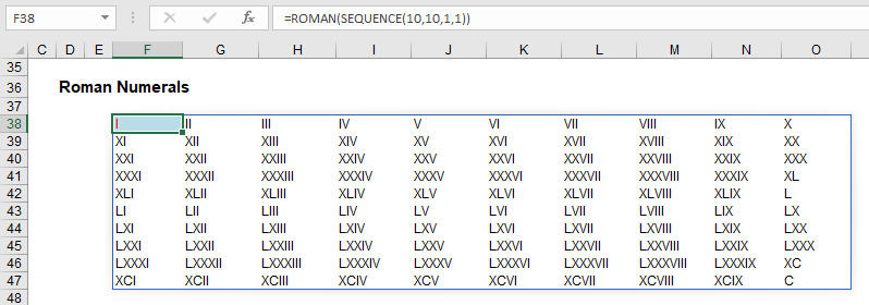
Some of my peers had fun combining it with the ROMAN function:

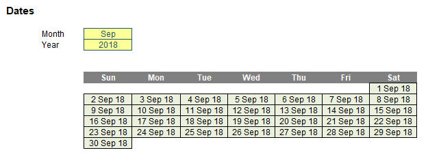
To my mind though, my favourite simple illustration is creating a monthly calendar. A little magic with the DATE and WEEKDAY functions combined with some conditional formatting and suddenly you have:

As mentioned above, SEQUENCE is arguably more powerful when included in a more complex formula. For example:

In this instance, I have created a grid using the Excel IPMT function to determine the amount of interest to be paid in each monthly instalment. Cells G62:R71 calculate each monthly amount and column T sums these amounts to calculate the annual interest payment, a figure that is nontrivial to compute. The whole table may be replaced by the formula in cell V62:

=IF($F62="","",-SUM(IPMT(Annual_Interest_Rate/Months_in_Year,
SEQUENCE(1,Months_in_Year,($F62-1)*Months_in_Year+1,1),
Borrowing_Term*Months_in_Year,Amount_Borrowed))).

I am not going to explain this, and let me tell you why. Our company, SumProduct, builds and reviews financial models for a living. We see terrible modelling practices established day in, day out. We proactively try to discourage these traits by emphasising that complex formulas should be stepped out and made transparent. Here, that can be done using the original table. I don’t want people using SEQUENCE, Dynamic Arrays, or other spilled formulas to wrap up complicated calculations into an opaque Pandora’s Box. Yes, calculation times may be slower. Live with it. Sometimes you need to see the scenery to appreciate the beauty. I’m just a little fearful that people will embrace these functions a little too readily, which could open the road to Excel hell.

On an upbeat note, I put a simple formula in cell G61:

=TRANSPOSE(SEQUENCE(Months_in_Year))

Yes, I am using TRANSPOSE without Ctrl+Shift+Enter. We are in new territory here.

As for the final function, RANDARRAY we go!

And so, to the final function for now: RANDARRAY. The RANDARRAY function returns an array of random numbers between 0 and 1. It’s not clear from Microsoft, but it’s my belief this is analogous to the pre-existing RAND function, which generates a number greater than or equal to zero and strictly less than one. It is noted, though, that RANDARRAY is different from the RAND function insofar that RAND does not return an array.

The function has the following syntax:

=RANDARRAY([rows], [columns])

The function has two arguments, both optional:

• rows: This specifies how many rows the results should spill over. If omitted, the default value is 1.
• columns: This specifies how many columns the results should spill over. If omitted, the default value is also 1.

Therefore, RANDARRAY() behaves like RAND().

Again, I’ll start with a basic demonstration:

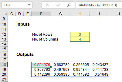
This can be useful for generating “seed” values for simulations analysis, for example. Anecdotal evidence suggests using RANDARRAY in a simulations formula rather than using a macro or Data Table may generate calculation speed efficiencies of greater than 50%. The jury is still out on this one, but it’s definitely worth exploring.

There is no RANDBETWEENARRAY function, but you can construct it yourself:

Here, in cell F44, I have used the formula

=ROUNDDOWN(RANDARRAY(H36,H37)*(H39-H38+1),0)+INT(H38)

to generate my equivalent RANDBETWEEN function. Since RANDARRAY generates a random number greater than or equal to zero and strictly less than one, ROUNDDOWN(RANDARRAY(H36,H37)*(H39-H38+1),0) generates a random integer (all equally likely) between zero and nine (this is 9, because the number generated is a whole number greater than or equal to zero but strictly less than 10 [10 – 1 + 1]). Since this is added to 1 (INT(H38)), the random whole number will be an integer between 1 and 10. Simple, if you have a maths Ph.D.

For a final example, imagine you are a schoolteacher and you have ten five-year-old children:

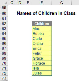
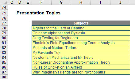
For each of the next ten weeks, you have topics you want one of them to present on:

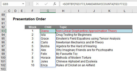
I can use RANDARRAY in tandem with SORTBY to determine a presentation order for the term:

The formula

=SORTBY(F63:F72,RANDARRAY(COUNTA(F63:F72)))

sorts the “Child” order randomly (and a similar formula is used for “Topic” too). In a past life, as an independent expert, I once had to attest that drug testing was being performed entirely randomly, ie, free from any material bias. SORTBY(RANDARRAY) dries up that well for me once and for all.

An Excel Evolution: The Series

Getting started

Part 1: Excel: Microsoft Unveils Dynamic Upgrades

Part 2: Excel: Arrays, Tables, and “The Twilight Zone”

Part 3: Excel: 2 New Errors and a SINGLE Function

Function focus

Part 4: This Excel Change is More Than SORT of a Big Deal

Part 5: Focus on 2 New Excel Functions: UNIQUE and FILTER

Part 6: Excel New Function Focus: SEQUENCE and RANDARRAY

Final thoughts

Part 7: Will Dynamic Arrays Kill Data Tables, PivotTables?

— Liam Bastick, FCMA, CGMA, FCA, is director of SumProduct, a global consultancy specialising in Excel training. He is also an Excel MVP (as appointed by Microsoft) and author of An Introduction to Financial Modelling. Send ideas for future Excel-related articles to him at liam.bastick@sumproduct.com. To comment on this article or to suggest an idea for another article, contact Jeff Drew, an FM magazine senior editor, at Jeff.Drew@aicpa-cima.com.