Will Dynamic Arrays kill Data Tables, PivotTables?

Editor’s note: Microsoft recently announced a partial rewrite of Excel’s calculation engine. This result is an evolutionary leap that promises to bring numerous improvements to Excel users in the coming years. Already unveiled are a new type of calculation (Dynamic Arrays), seven new functions, and two new errors. These changes have not yet been rolled out to all Excel users, but you don’t have to wait to see what they can do. Excel MVP Liam Bastick is covering all the changes in a seven-part series. In this final instalment, Bastick explores the impact Dynamic Arrays could have on other features/tools in Excel.

The first six articles of this series have covered everything I uncovered working with Excel’s new Dynamic Arrays toolset in preview mode. This article is not going to rehash what was written in those first six articles. Instead, we are ending this journey with an interesting note or two. There are some significant ramifications for Excel, once these seven new functions and Dynamic Arrays features roll out and become Generally Available (this does assume the “final” versions of everything highlighted in the series do not change drastically).

Let me explain.

I begin with a two-dimensional Data Table (Alt+D+T) with an old favourite for this sort of thing, calculating monthly payments on various loan amounts over various durations.

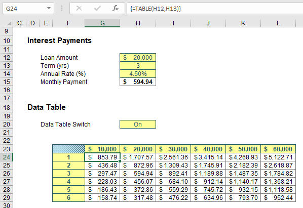
I have no plans to go through Data Tables here, suffice to say they are a great tool for “what-if?” analysis, albeit they can consume vast quantities of memory. This summary table shows how the monthly instalments would vary for different terms (in years) and different amounts borrowed.

Now, take a look at using three Dynamic Array formulas:

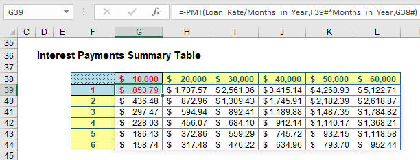
Can you spot the difference? In the second table, I have highlighted three cells:

• G38 contains the formula =SEQUENCE(1,6,10000,10000).
• F39 contains the formula =SEQUENCE(6).
• G39 contains the formula =-PMT(Loan_Rate/Months_in_Year,F39#*Months_in_Year,G38#). See how using the Spilled Range Operator (“#”) makes all the difference?

That’s it! Now, I am not saying all Data Tables may be replaced by Dynamic Array formulas, but can you see the future? And guess what, it doesn’t stop there. Let me replicate one feature in Excel many of us are familiar with: the PivotTable.

In this illustration, I have created a 1,200-record table (Ctrl+T):

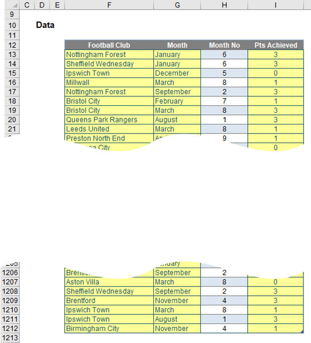
It’s all made up of randomly generated data, and you will just have to guess whom I support. The important thing to note is I have created a table, called Football_Data, so I may add records and the table will extend automatically.

Next, I created a “Pseudo PivotTable”:

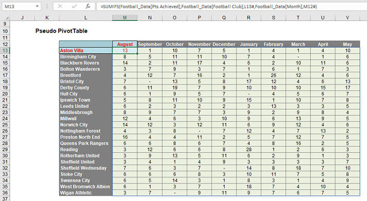
This was created using three Dynamic Array formulas (again, highlighted):

• M12 contains the formula =TRANSPOSE(UNIQUE(SORTBY(Football_Data[Month],Football_Data[Month No]))), which sorts the months into the required order.
• L13 contains the formula =SORT(UNIQUE(Football_Data[Football Club])), which simply sorts the clubs into alphabetical order.
• M13 contains the formula =SUMIFS(Football_Data[Pts Achieved],Football_Data[Football Club],L13#,Football_Data[Month],M12#), which spills out the points earned each month using a standard SUMIFS formula and the Spilled Range Operator (“#”).

Think about it. I have created a formulaic PivotTable that calculates no discernibly slower than the real thing. However, the source data may be extended, values may change, and I don’t need to hit “Refresh”. Is this the end for PivotTables?

It’s easy to get carried away. Dynamic Array formulas make league tables a breeze:

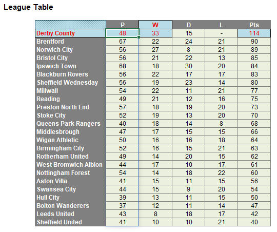
However, rather than get sidetracked, I’d rather stay “on track” with PivotTables and finish this section unpivoting the PivotTable we have just created (the references have changed as they are on a different worksheet in my example):

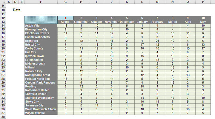
Unpivoting can be a nightmare, but it is possible. You don’t need to use Dynamic Arrays to do it, but I will to showcase them:

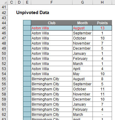
There is a hidden formula in cell E45. You can see why it is hidden — for those of you with a nervous disposition, please look away now:

=INDEX(SORT(G12#&" - "&F14:F37),ROUNDUP(SEQUENCE(COUNTA(F14:F37)
*COUNT(G12#))/COUNT(G12#),0),MOD(SEQUENCE(COUNTA(F14:F37)*COUNT(G12#))
-1,COUNT(G12#))+1)

Oh dear. That’s a horror. Rather than write 1,000 words trying to explain this, let me detail the concept instead. SORT(G12#&" - "&F14:F37) provides every combination of Month Number concatenated with a Football Club, separated by a “ – ” delimiter, eg:

1 – Aston Villa, 2 – Aston Villa, …, 10 – Aston Villa, 1 – Birmingham City, 2 – Birmingham City, …

The problem is SORT(G12#&" - "&F14:F37) spills this into a 10-column by 24-row array. I want it as a list, so the entire rest of the formula simply forces the array down a column of 240 rows instead. INDEX is used to locate the next record in the array, with contrived formulas to determine the row and column numbers of the virtual grid.

SUMIFS is used to create the points total for each row, and to be honest, simpler formulas could have been used elsewhere, too. But that’s my point. As I have written this series, it’s hard not to get carried away with all this and try to do everything in Dynamic Arrays. I have worked for years with Excel and been a keen advocate for keeping everything simple. Dynamic Arrays scare me that we may not help ourselves and write monsters like the formula above.

Maybe Excel’s simpler functions and features will live on after all.

Concerns about calculation order

If it feels as if you have aged a year since you started reading this series, you probably have. There’s a lot to get excited about, and I have highlighted some of the issues, too — many of which I am sure will be ironed out by the time everything becomes Generally Available. However, I am not sure the following concern will be going away anytime soon.

When I calculate something in Excel, if I use the same formula, I must get the same answer, right? Well — not necessarily. Consider the following:

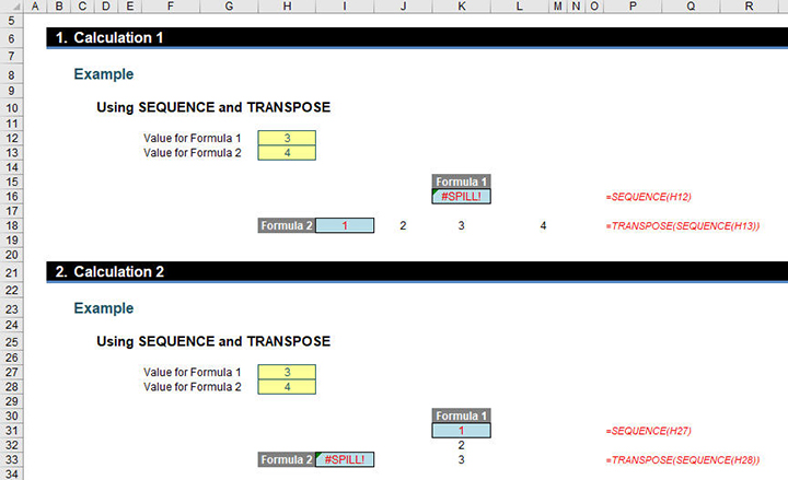
In the example above, Calculations 1 and 2 are identical but deliver different results (ie, different #SPILL! errors). Why?

• In Calculations 1 and 2, both values for Formula 1 (cells H12 and H27) and Formula 2 (cells H13 and H28) were originally set to 1. This causes no #SPILL! errors.
• In Calculation 1, the value for Formula 2 (cell H13) was then changed to 4 with no error.
• Then, in Calculation 1, the value for Formula 1 (cell H12) was changed to 3. This caused the resultant #SPILL! error in cell K16.
• Next, in Calculation 2, the value for Formula 1 (cell H27) was changed to 3 with no error.
• Then, in Calculation 2, the value for Formula 2 (cell H28) was changed to 4. This caused the resultant #SPILL! error in cell I33.

I am not sure what the solution is for this problem. Technically, #SPILL! is working correctly, but it doesn’t seem right that two results may be generated in this instance depending upon what input I change first. The jury is out on this one.

Word to the wise

As of this of writing, all the features, functions, and error messages covered in this series are beta features only. They are available to a portion of Office Insiders at this time, but don’t let that put you off. Start getting excited now! Microsoft will continue to optimise these features over the next several months. This means they might change. When they’re fully cooked, Microsoft will release them out into the wild, first to all Office Insiders and then finally to Office 365 subscribers (this is when a feature is known as “Generally Available”).

The future’s looking bright though.

An Excel Evolution: The Series

Getting started

Part 1: Excel: Microsoft Unveils Dynamic Upgrades

Part 2: Excel: Arrays, Tables, and “The Twilight Zone”

Part 3: Excel: 2 New Errors and a SINGLE Function

Function focus

Part 4: This Excel Change Is More Than SORT of a Big Deal

Part 5: Focus on 2 New Excel Functions: UNIQUE and FILTER

Part 6: Excel New Function Focus: SEQUENCE and RANDARRAY

Final thoughts

Part 7: Will Dynamic Arrays Kill Data Tables, PivotTables?

— Liam Bastick, FCMA, CGMA, FCA, is director of SumProduct, a global consultancy specialising in Excel training. He is also an Excel MVP (as appointed by Microsoft) and author of Introduction to Financial Modelling. Send ideas for future Excel-related articles to him at liam.bastick@sumproduct.com. To comment on this article or to suggest an idea for another article, contact Jeff Drew, an FM magazine senior editor, at Jeff.Drew@aicpa-cima.com.