In Excel, INDEX MATCH is a winning combination

Last month, we looked at VLOOKUP and HLOOKUP and saw that these functions do not always behave as you would expect. They are less flexible when you want to return a corresponding value in a noncontiguous range (eg, on another worksheet in another workbook). Therefore, this month’s column looks at a more flexible alternative.

Let’s start with an example. When preparing financial statements in Excel, you might wish to construct a formula that highlights balancing errors in the Balance Sheet, reporting the first period during which the misbalance occurs.

In the illustration below, row 15 has a formula that produces a value of one (1) if Net Assets (row 11) does not equal Total Equity (row 13) and a value of zero (0) otherwise. This is called reporting by exception, as only errors are flagged (ie, given a nonzero value). It’s a simple way of determining how many errors you have. I have used conditional formatting, number formatting, and the Wingdings font to dress these values up as green-shaded ticks and red-shaded crosses, but that’s another story for another day.

I want to find the first error value (ie, a “1”) and report back the corresponding month ending date from row 5. This is a common modelling query. The usual suspects, LOOKUP and HLOOKUP/VLOOKUP, do not work here:

• LOOKUP(lookup_value, lookup_vector,[result_vector]) requires the balance checks to be in ascending order (ie, ascending alphanumerically, duplicates allowed) — that is not the case here; whilst
• HLOOKUP(lookup_value,table_array,row_index_number,[range_lookup]) gives #VALUE! since the first row must contain the data to be “looked up”, but the Balance Check is in row 15 in our example above, whereas the dates we need to return are in row 5. Hence, we get a syntax error.

There is a solution, however: INDEX MATCH. The two functions form a highly versatile tag team but are worth introducing individually.

INDEX

Essentially, INDEX(array, row_number,[column_number]) returns a value or the reference to a value from within a table or range (list).

For example, INDEX({7,8,9,10,11,12},3) returns the third item in the list {7,8,9,10,11,12}, ie, 9. This could have been a range: INDEX(A1:A10,5) gives the value in cell A5, etc.

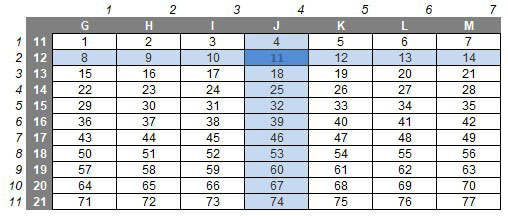
INDEX can work in two dimensions as well (hence the column_number reference). Consider the following example:

INDEX(G11:M21,2,4) returns the value in the second row, fourth column of the table array G11:M21 (clearly 11 in the above illustration).

MATCH

MATCH(lookup_value,lookup_array,[match_type]) returns the relative position of an item in an array that (approximately) matches a specified value. It is not case sensitive.

The third argument, match_type, does not have to be entered, but for many situations, I strongly recommend that it is specified. It allows one of three values:

• match_type 1 [default if omitted]: Finds the largest value less than or equal to the lookup_value, but the lookup_array must be in strict ascending order, limiting flexibility;
• match_type 0: Probably the most useful setting. MATCH will find the position of the first value that matches lookup_value exactly. The lookup_array can have data in any order and even allows duplicates; and
• match type -1: Finds the smallest value greater than or equal to the lookup_value, but the lookup_array must be in strict descending order, again limiting flexibility.

When using MATCH, if there is no (approximate) match, #N/A is returned (this may also occur if data are not correctly sorted depending upon match_type).

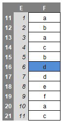
MATCH is fairly straightforward to use:

In the figure above, MATCH(“d”,F11:F21,0) gives a value of 6, being the relative position of the first “d” in the range. Note that having match_type 0 here is important. The data contain duplicates and are not sorted alphanumerically. Consequently, match_types 1 and -1 would give the wrong answer: 7 and #N/A, respectively.

INDEX MATCH

Whilst useful functions in their own right, INDEX and MATCH form a highly versatile partnership when combined. Consider our original problem:

MATCH(1,J15:U15,0) equals 5, ie, the first period the balance sheet does not balance in is Period 5. But we can do better than that.

INDEX(J5:U5,5) equals May-19, so combining the two functions:

=INDEX(J5:U5,MATCH(1,J15:U15,0))

equals May-19 in one step, giving us the first period of misbalance.

Note how flexible this combination really is. We do not need to specify an order for the lookup range; we can have duplicates, and the value to be returned does not have to be in a row/column below/to the right of the lookup range. (Indeed, it can be in another workbook, never mind another worksheet!)

With a little practice, the above technique can be extended to match items on a case-sensitive basis, use multiple criteria, and even “grade”. The attached Excel workbook provides several examples as illustrations.

— Liam Bastick, FCMA, CGMA, FCA, is director of SumProduct, a global consultancy specialising in Excel training. He also is an Excel MVP (as appointed by Microsoft) and author of the book Introduction to Financial Modelling. Send ideas for future Excel-related articles to him at liam.bastick@sumproduct.com. To comment on this article or to suggest an idea for another article, contact Jeff Drew, an FM magazine senior editor, at Jeff.Drew@aicpa-cima.com.