


Editor’s note: This article is Part 2 of a three-part introduction to Python in Excel. It’s an important feature in Excel allowing you to use more advanced data analytics, complex visualisations, machine learning, and automation. The series details Python’s functionality and application for data analysis — a highly relevant skill for today’s accounting and finance professionals. Part 1 provides an overview of the topic and details how Python code may be inserted into Excel. Part 3 looks at errors and more complex examples using imported libraries and modules.
This second article in the series is split into three sections:
- Working with lists: When using Python in Excel to analyse data, one of the simplest ways of storing data is in a list. This section highlights some of the key items to consider.
- Extending the idea with (dynamic) arrays: Extrapolating the list idea, using the Python library NumPy allows arrays to be defined more extensively. This section provides further details.
- Using Python in Excel to reference Excel entities: Discusses how Python works specifically with Excel data sources such as an Excel Table, a Power Query Table, or a defined name or dynamic array, with or without headers.
Working with lists
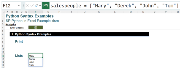
When using Python in Excel to analyse data, one of the simplest ways of storing data is in a list. The following image shows a simple list of employees, shown in the Excel Value view:
The Python code used is:
salespeople = [“Mary”, “Derek”, “John”, “Tom”]
This creates a list of spilled values, which Python identifies as salespeople, namely Mary, Derek, John, and Tom.
By assigning a variable, salespeople, to the output, this variable may be referenced when creating code in other cells. This is good practice when creating Python code. There are some rules for these variable names — they:
- Are case-sensitive.
- Only contain letters, numbers, and underscores (_).
- Must begin with a letter or an underscore, never a number.
- Must not be the same as a keyword in Python, eg, “True”.
Variables will be utilised whenever Python code is created.
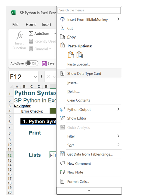
Since the currently selected view is Excel Value, the result is a dynamic array spilling from cell F12. Changing the view of the result to Python Object, the object appears as a list object:
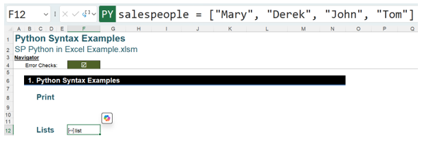
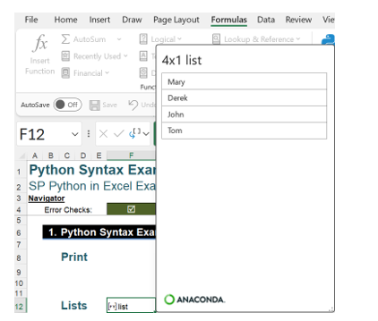
It is possible to see the data by right-clicking and selecting Show Data Type Card.
This shows the data in the list.
Note that the variable identifying the list, salespeople, is not shown. This identifier may be referenced in other Python code. For example, the code to show the list with an extra employee will be entered in cell H12. The Excel Value view has been selected for F12 and H12 to make it easier to follow:
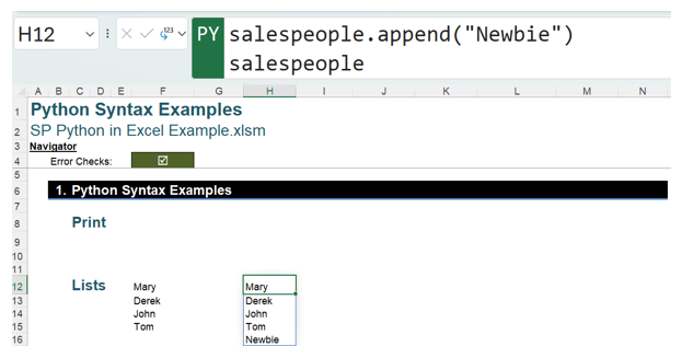
The Python code used is:
salespeople.append(“Newbie”)
salespeople
This adds the field Newbie to the end of the list salespeople and then outputs the extended salespeople.
Extending the idea with (dynamic) arrays
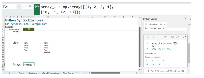
The Python library NumPy allows arrays to be defined. It is preinstalled in the Excel frontend and has the short name np. The next image shows a simple 4×2 (four columns by two rows) array in the Excel Value view:
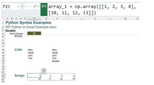
The Python code used is:
array_1 = np.array([[1, 2, 3, 4],
[10, 11, 12, 13]])
Using the Python view, this has returned a new Python Object, called an ndarray, which is a multi-dimensional array of items of the same type and size. You should note that the Python Editor has been opened to show the values in the ndarray.
To see this as two columns instead, the values may be entered in pairs:
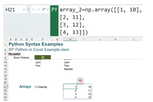
The Python code used is:
array_2=np.array([[1, 10],
[2, 11],
[3, 12],
[4, 13]])
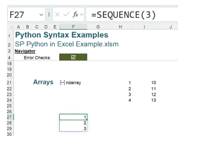
The NumPy library allows operations on matrices to be performed. Two very simple dynamic arrays will be created. The first is created using the Excel dynamic array formula:
=SEQUENCE(3)
This gives a column of numbers starting in cell F27:
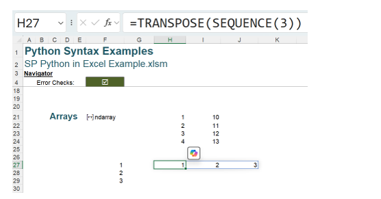
Similarly, a row of numbers may be created:
=TRANSPOSE(SEQUENCE(3))
Referring to these arrays, we use the # notation, which cites only the top left-hand cell in the dynamic array range. Therefore, using Python code, the arrays may be combined:
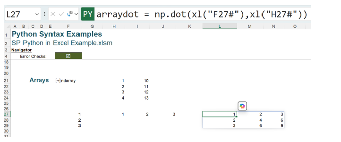
arraydot = np.dot(xl(“F27#”),xl(“H27#”))
This gives a 3×3 array, where the values have been multiplied. If the calculation involves a vector (either one row or one column) and an array, then the vector must come first to avoid Python errors:
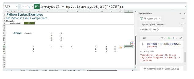
arraydot2 = np.dot(arraydot,xl(“H27#”))
The error is:
ValueError: shapes (3,3) and (1,3) not aligned: 3 (dim 1) != 1 (dim 0)
If the vector appears first, no errors are produced. The result is shown using the view Excel Value:
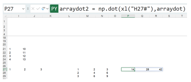
A matrix vector calculation has been performed, using the Python code
arraydot2 = np.dot(xl(“H27#”),arraydot)
where arraydot is the 3×3 matrix:

The resulting vector,

is calculated by adding the products of each value in the column of arraydot and the vector (dynamic array) identified by H27#:
1×1 + 2×2 + 3×3 = 14
1×2 + 2×4 + 3×6 = 28
1×3 + 2×6 + 3×9 = 42
More simple arithmetic may be performed with matrices. To show the vector arraydot2 as decimals instead, multiply each value by 0.01:
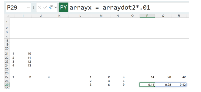
The Python code for this is:
arrayx = arraydot2*.01
where arrayx identifies the new vector. Using the NumPy library functions facilitates the manipulation of massive arrays of data in exactly the same way.
Using Python in Excel to reference Excel entities
The Python function that works specifically with Excel data sources is:
xl(“source”, headers = True/False)
The source can be a range, Excel Table, Power Query Table, defined name, or dynamic array, with or without headers. The output is read into a DataFrame object.
Since it is good practice to specify a variable to assign to the DataFrame object, the syntax used is:
x=xl(“source”, headers = True/False)
where x is the variable.
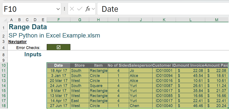
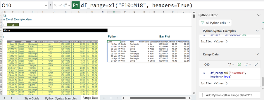
The example below uses a contiguous range as the data source. The range the data is extracted from is F10:M18:
Since the source is Excel data, the variable names may be given the prefix df (for DataFrame). This will allow the distinction between Python objects and Excel formulae.
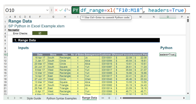
The formula used is:
df_range=xl(“F10:M18”, headers=True)
This extracts the data in F10:M18 into a DataFrame, which may be identified as df_range. This is initially shown as a DataFrame:

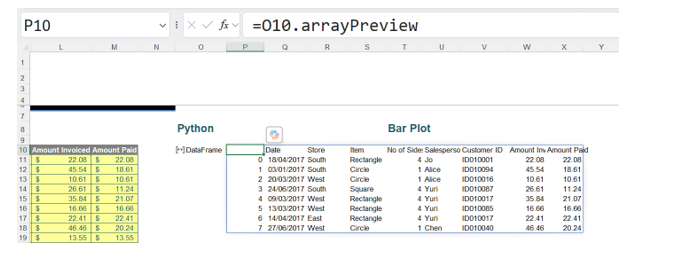
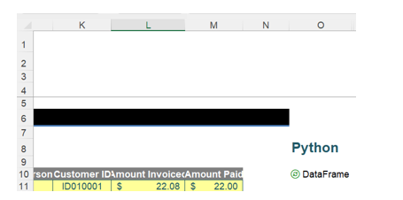
The Excel data may be viewed by using the Excel Value view:
Another way to see the Excel data is to click in the cell containing the DataFrame to access the Insert Data icon:

Clicking on the Insert Data icon gives more options:
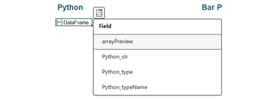
Choosing arrayPreview allows the insertion of a preview of the Excel data in the workbook:
To see a temporary preview of the Python DataFrame, the PY icon may be clicked:
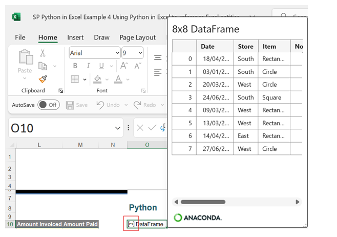
This shows more details about the data in a tabular form. The card is also accessible by right-clicking on the DataFrame and selecting Show Data Type Card:
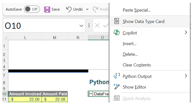
The Python objects are recalculated when any of the underlying data is changed (see more about this below). Therefore, by changing data in the range F10:M18 in the current example, it is possible to see the DataFrame df_range refreshing. Below, Amount Paid in cell M11 has been changed from $22.08 to $22.00. Note the refresh icon:
If other DataFrames were using df_range, then this would cause them to recalculate, too.
However, Python cells will only refer to DataFrames above and/or to the left of the current cell. If we try to refer to the DataFrame created in cell O10 from cell O8, we receive the following message:
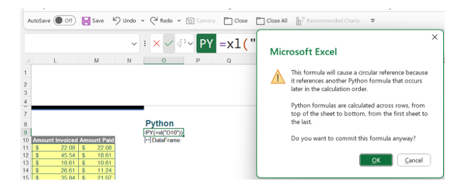
If we click OK, we get a firm rejection of the formula:

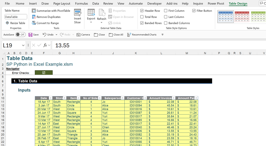
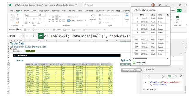
Ranges of data have been selected by specifying cell references so far, but Python can also read all data from an Excel Table. The Table on the Table Data sheet is named DataTable:
Python recognises the Table name within the xl() function. The data card is shown in the following image in order to show the number of rows and columns in the DataFrame:
The Python formula is:
df_Table=xl(“DataTable[#All]”, headers=True)
If the data in the Table is changed, for example by inserting a row, then df_Table will recalculate. Note the row has appeared on the Data Type Card, and the number of rows in total is now 1001 (the header, plus 1,000 rows numbered zero [0] to 999):
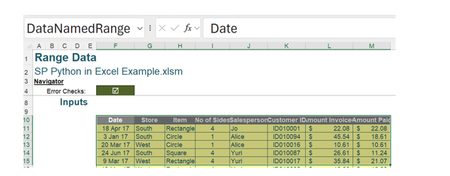
The Python xl() function will also recognise a named range and extract the data.
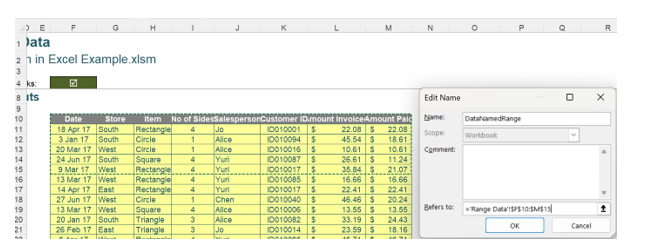
A named range may contain a range of cells. A named range DataNamedRange has been created for cells F10:M15 below.
Named ranges may be viewed using the Name Manager on the Formulas tab:

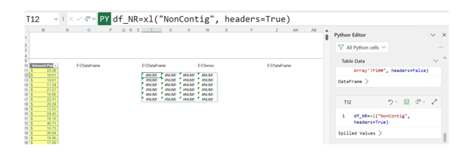
The Table DataTable also appears in the Name Manager. Note that new named ranges may also be created from here. It is possible to create a named range for noncontiguous cells:
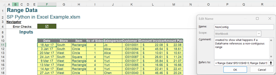
Whilst this used to cause errors if referenced by Python, it is now an acceptable way of referencing more than one contiguous range in a DataFrame. Considering the named range DataNamedRange:
Data may be extracted from this range into a DataFrame:
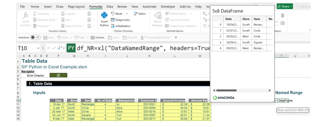
This uses the Python formula:
df_NR=xl(“DataNamedRange”, headers=True)
The following image shows what happens if the NonContig range containing noncontiguous data is used:

In earlier releases of Python in Excel, this caused an Excel resources error, but now this may appear to be a way to reference noncontiguous ranges in DataFrames. However, if the Excel Value view is used:
The values cannot be displayed, and the card is equally confusing:
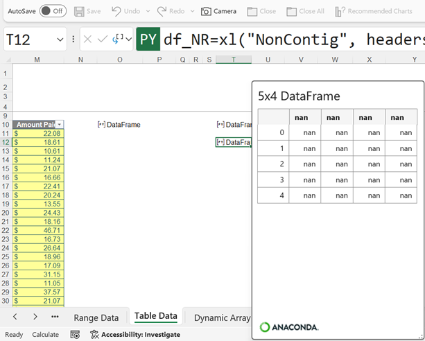
NaN (Not a Number) values are also called missing values, which means that this data cannot be processed. The Python xl() function also recognises dynamic arrays. This example uses the following dynamic array:
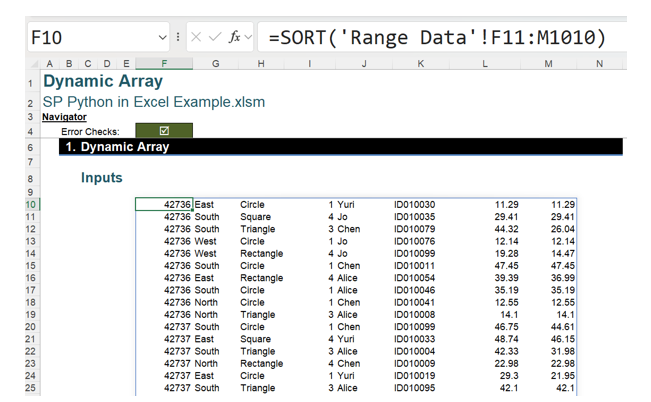
This dynamic array may be extracted to a DataFrame. The dynamic array is identified by cell reference F10#:
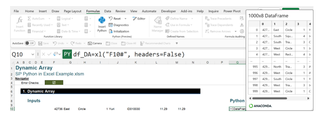
The Python formula here is:
df_DA=xl(“F10#”, headers=False)
Note that, although for this example the Python formula accesses Excel data in the same sheet, data from other sheets may be extracted:

This applies to all the Excel entities accessed in DataFrames. Queries created in Power Query may also be used as data sources for Python. This query will be used as a source for the next Python example:
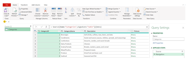
In the next image, the DataFrame and card for this query are shown:
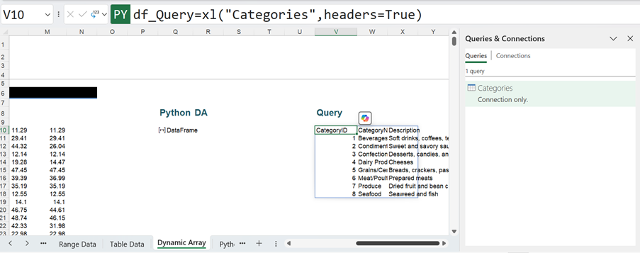
The Python formula here is:
df_Query=xl(“Categories”,headers=True)
Using queries is the recommended method for accessing external data sources for Python, although it may be used for cleaning and transforming data.
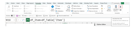
Other Python DataFrames may be referenced either by using the DataFrame name or the cell location. Here, on the Table Data sheet, df_Table has been used as the source, and the new DataFrame, df_Item, includes the Item column. Note that since there is only one column, a special DataFrame called a Series is created.

The formula is:
df_Item=df_Table[‘Item’]
or
df_Item=xl(“O10”)[‘Item’]
As previously stated (in Part 1 of the series), Python formulae recalculate automatically in row-major order when a value used in a Python formula is changed. This means across row 1 from A to XFD and then row 2 and so on. If this automation becomes a problem, with the premium version of Python it can be controlled from the Calculation Options settings in the Formulas tab:

Choosing Partial will currently suspend the automatic calculations for Python and Data Tables. There are three ways to manually recalculate Python when the workbook is set to Partial or Manual:
1. Use the keyboard shortcut F9.
2. Go to Calculate Now on the Formulas tab.
3. Go to a cell with a stale value (which can be activated using Format Stale Values), displayed with strikethrough formatting, and select the error symbol next to that cell. Then select Calculate Now, as in the previous point.
— Liam Bastick, FCMA, CGMA, FCA, is director of SumProduct, a global consultancy specialising in Excel training. He is also an Excel MVP (as appointed by Microsoft) and co-author of Python in Excel: Unlocking Powerful Data Analysis and Automation Solutions. Send ideas for future Excel-related articles to him at liam.bastick@sumproduct.com. To comment on this article or to suggest an idea for another article, contact Oliver Rowe at Oliver.Rowe@aicpa-cima.com.

